Multi-layer perceptron: Hyperparameter tuning
October 12, 2025
This week, we will learn about how to build a multi-layer perceptron (MLP), as well as hyperparameter tuning and debugging the model. Some information may be duplicate from previous posts, but I will go over it again to keep the posts on MLPs self-contained.
What is a multi-layer perceptron (MLP)?
A MLP is a artificial feedforward neural network that consists on multiple layers including an input layer, hidden layers (at least one), and an output layer. The layers are fully connected, which means that each neuron in layer a is connected to each neuron in layer b. Each connection is assigned a weight and each neuron a bias.
There are two phases when training a MLP: forward propagation and backward propagation. During forward propagation, the data flows from the input layer, through all the intermediate layers, and finally through the output layer with each layer processing the outputs of the previous one. The output is then compared to the truth and the error is calculated. During backpropagation, the error flows backwards through the layers, adjusting the weights and biases using techniques such as gradient descent, which tries to find the combinations of weights and bias that minimize the error. Once this process finishes for all weights and biases, the model will once again switch to forward propagation.
We will be using the California housing dataset we discussed last week to train and evaluate our model. This dataset contains aggregated data regarding each district in California such as median income, population, and location (latitude and longitude). For more information see this post.
Since we already went over the dataset in the last post, we can jump straight into the model and experiments. Our model class contains the following constructor (minus the docstring):
class MLP(nn.Module):
    def __init__(self, input_dim, hidden_dim, dropout):
        super().__init__()
        self.net = nn.Sequential(
            nn.Linear(input_dim, hidden_dim),
            nn.ReLU(),
            nn.Dropout(dropout),
            nn.Linear(hidden_dim, hidden_dim),
            nn.ReLU(),
            nn.Linear(hidden_dim, 1),
        )
Let’s break it down:
nn.Sequential
- This simplies building a neural network by organizing the layers in a sequential order. In other words, the network knows that it has to flow sequentially through the layers in the order defined.
nn.Linear(input_dim, hidden_dim)
- This is a fully connected linear layer with input size input_dim (output of CNN) and output size of hidden_dim neurons.
- This is a fully connected linear layer with input size input_dim (output of CNN) and output size of hidden_dim neurons.
nn.ReLU()
- This is a Rectified Linear Unit activation function. It is defined as $\text{ReLU}(x) = \text{max}(0, x)$. Essentially, it zeros out the negative values while introducing non-linearity. This type of activation function is simple and fast to use compared to others such as $\text{tanh}(x)$ or sigmoid.
- This is a Rectified Linear Unit activation function. It is defined as $\text{ReLU}(x) = \text{max}(0, x)$. Essentially, it zeros out the negative values while introducing non-linearity. This type of activation function is simple and fast to use compared to others such as $\text{tanh}(x)$ or sigmoid.
nn.Dropout()
- This randomly turns off neurons (equivalent to zeroing out some inputs), forcing the network to learn more general features instead of relying solely on specific neurons.
nn.Linear(hidden_dim, hidden_dim)
- This is another fully connected linear layer, but now the input size is hidden_dim and the output size is hidden_dim. This implies this is an intermediate layer.
- This is another fully connected linear layer, but now the input size is hidden_dim and the output size is hidden_dim. This implies this is an intermediate layer.
nn.ReLU()
- Same as before.
- Same as before.
nn.Linear(hidden_dim, 1)
- This is another fully connected linear layer, but now the input size is input_dim and the output size is $1$, which means we want to predict one scalar output per input.
- This is another fully connected linear layer, but now the input size is input_dim and the output size is $1$, which means we want to predict one scalar output per input.
As we can see, the model is pretty straightforward. I purposely made the hidden_dim and dropout variables because we will be varying this when tuning hyperparameters.
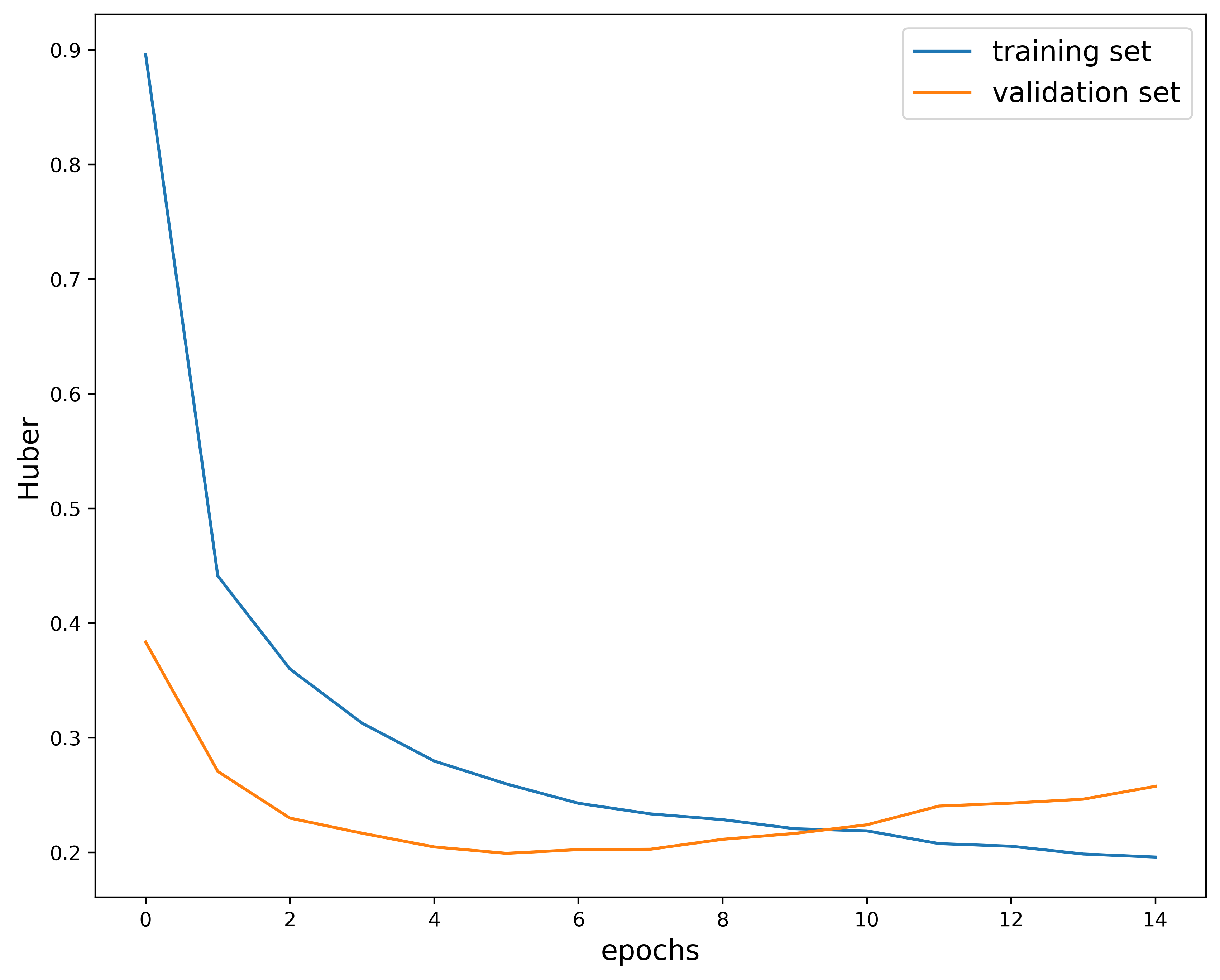
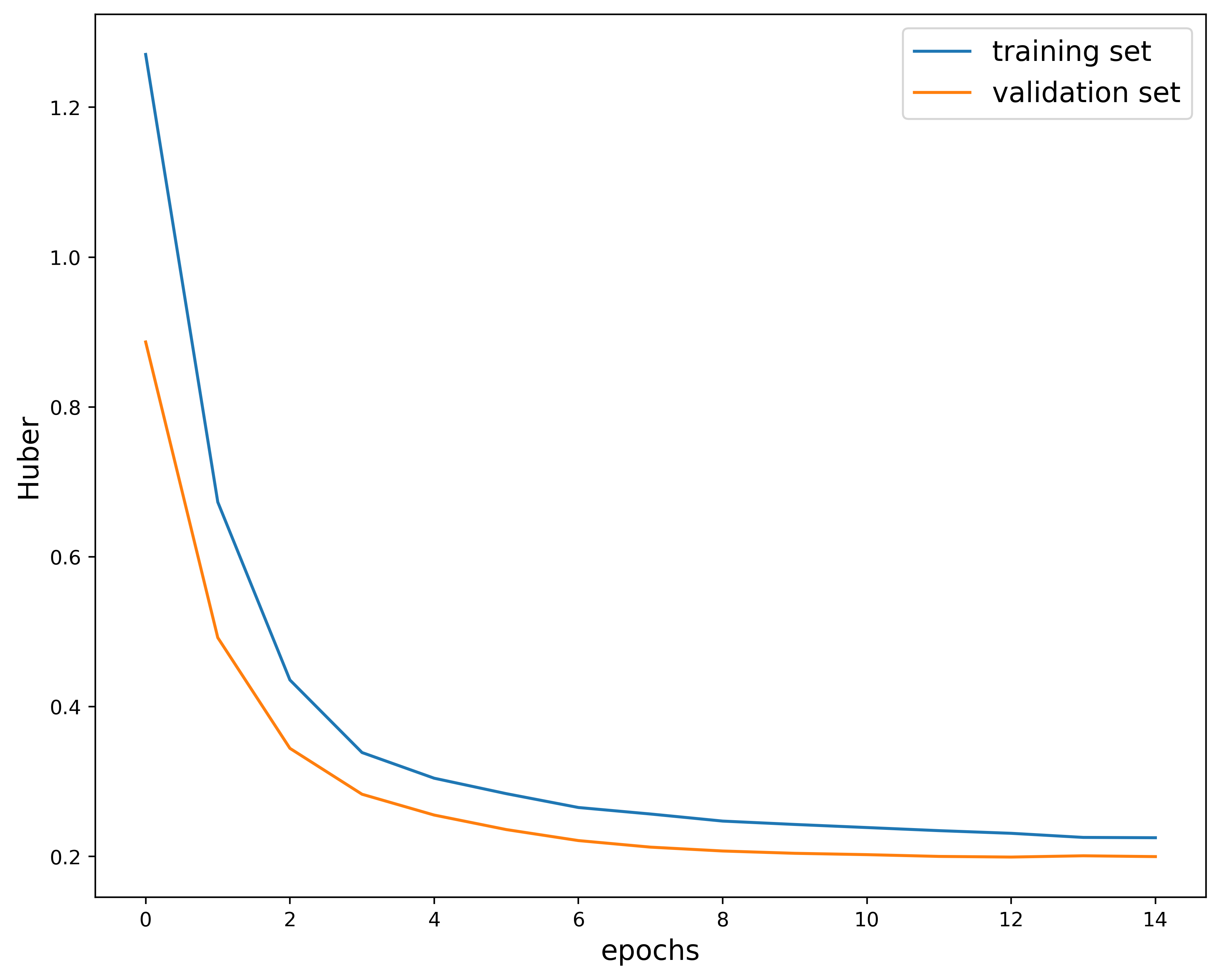
Training the model over $15$ epochs gives us the following:
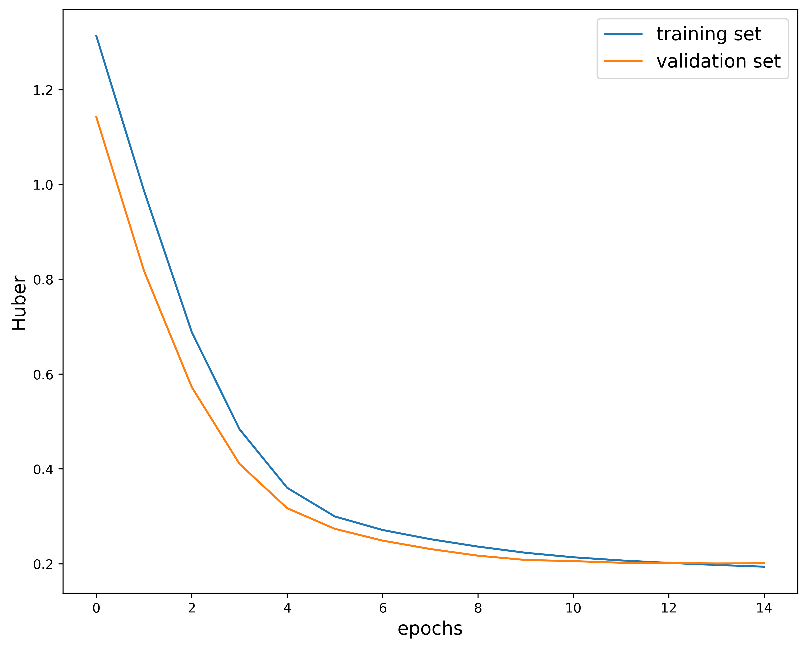
This plot shows how the Huber loss function varies over epochs in the training and validation phase. I used the Huber loss function as a metric because it is less sensitive to outliers when compared to the Mean Square Error. It is quadratic at small distances and linear for larger values.
The overall structure of the plot mostly looks good. Both the training and validation decrease as the model is trained. The only issue is with the higher epochs, where the curves end up crossing. This indicates that the model is most likely overfitting. You don’t want the validation metric to start cross the training metric since this implies that the model is no longer generalizing.
We can in fact check where the model started overfitting by looking in the “metrics_output.log” file generated at each run. This is the latter part of the file:
Epoch 11:
New best model at epoch 11 (val_loss=0.2057)
Train - Huber: 0.2138, R2-score: 0.6054
Validation - Huber: 0.2057, R2-score: 0.6258

Epoch 12:
New best model at epoch 12 (val_loss=0.2023)
Train - Huber: 0.2071, R2-score: 0.6200
Validation - Huber: 0.2023, R2-score: 0.6355

Epoch 13:
Train - Huber: 0.2019, R2-score: 0.6317
Validation - Huber: 0.2024, R2-score: 0.6378

Epoch 14:
New best model at epoch 14 (val_loss=0.2007)
Train - Huber: 0.1977, R2-score: 0.6416
Validation - Huber: 0.2007, R2-score: 0.6443

Epoch 15:
Train - Huber: 0.1939, R2-score: 0.6510
Validation - Huber: 0.2013, R2-score: 0.6450

Test - Huber: 0.2135, R2-score: 0.6071
Looking in this file, we see assume that the model started overfitting around epoch $13$ since this was the first instance of no new best model recorded. The solution would be to train the model for $12$ epochs instead of $15$. Essentially, the model will see the data less so it will not be able to overfit on the features. You can also include something like early stopping so that the training stops when the loss is no longer changing above some tolerance. Another technique is to use a scheduler to change the learning rate (or other hyperparameters) at scheduled intervals. This will help improve how your model generalizes.
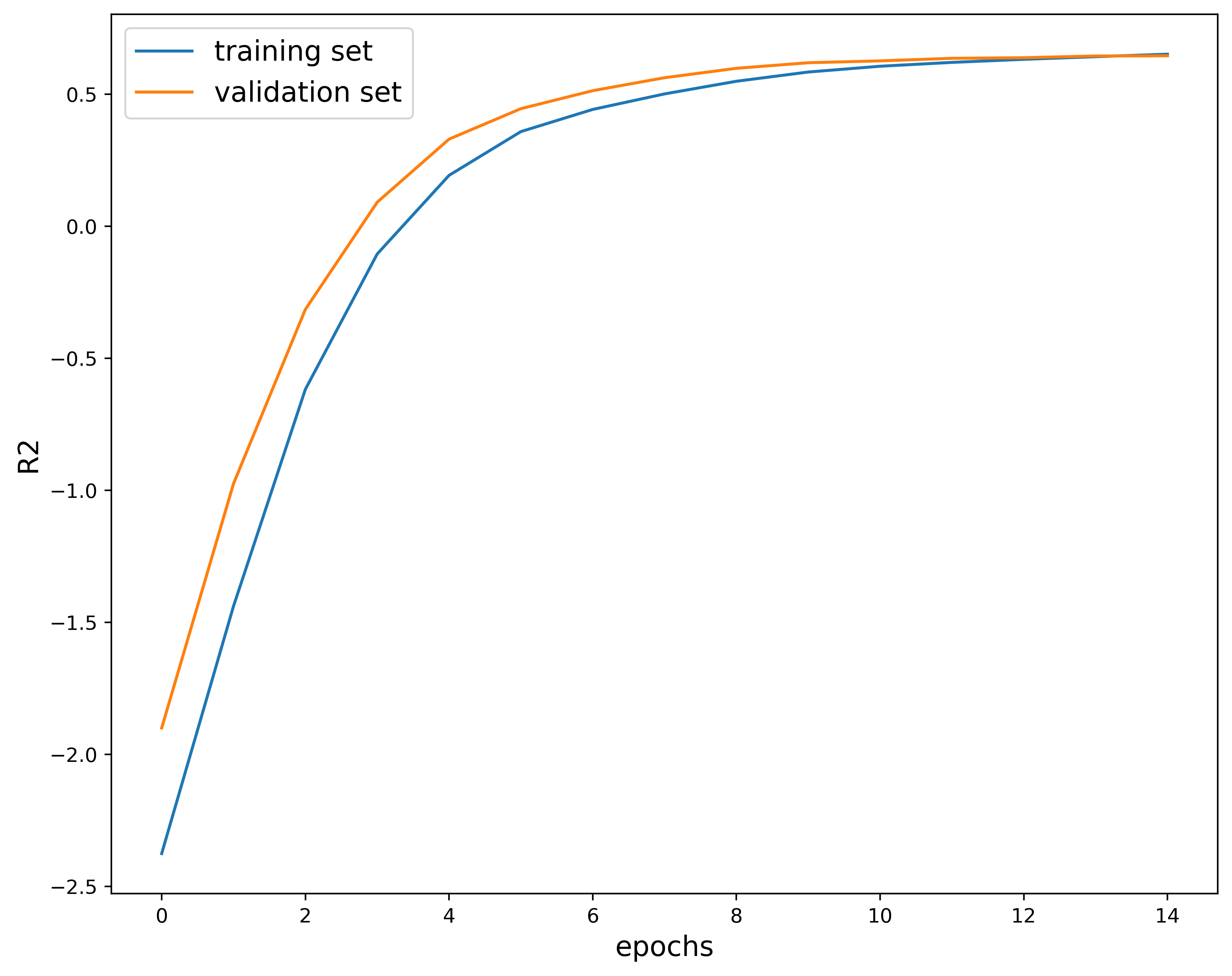
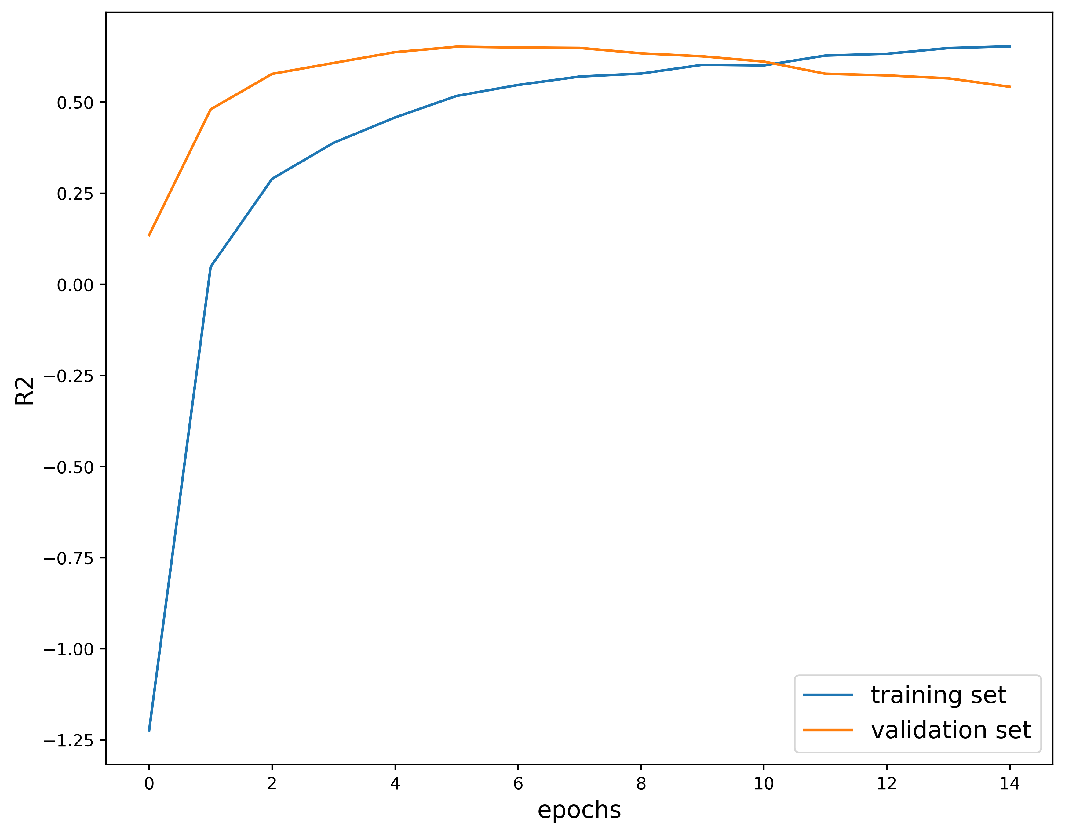
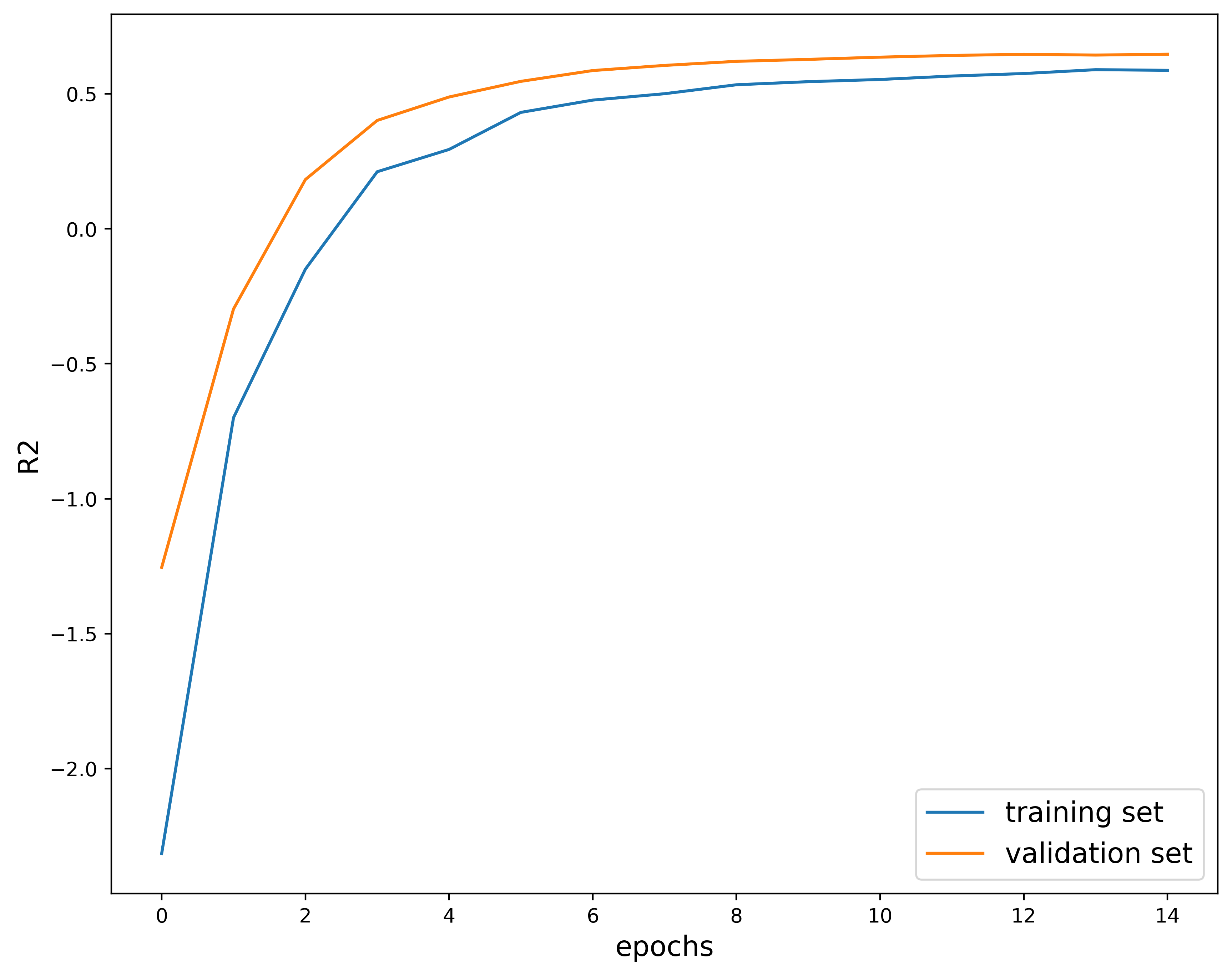
This next plot shows the $R^2$ score, which measures how well a regression model describes the variability of the target variable. In other words, it tells you how much of the variation in the target variable is explained by the inputs. This quantity is useful because it tells you how much of the variance in the predicted value is explained by the features or is just random noise. This value is bounded between $[-1, 1]$. Generally, a $R^2$ score closer to $1$ implies a better-fitting model. On the other hand, a value close to $0$ means that the model is not learning any of the patterns in the dataset, but can still output the average. On the opposite end of the spectrum, a score closer to $-1$ indicates a model that is doing worse than predicting the average. In fact, it is learning all the wrong things. In this case, the $R^2$ score appears to be close to $1$ so we can infer that the model is making well-informed predictions.
The results plots above are obtained by running the “base” model. The parameters used here are:
{
"model_version": "baseline",
"epochs": 15,
"learning_rate": 0.0001,
"hidden_dim": 64,
"dropout": 0.0
}
and can be found in .../experiments/base_model/params.json.
We can now check the logs generated when the code is ran once. In this case, the code generates a file called “grad_norm_output.log” located in .../experiments/base_model/. This file has information of what the gradient norm was across different layers at each epoch. For example:
Epoch: 11, grad_norm/net.0.weight: 0.2753058969974518
Epoch: 11, grad_norm/net.0.bias: 0.0689358115196228
Epoch: 11, grad_norm/net.3.weight: 0.27505698800086975
Epoch: 11, grad_norm/net.3.bias: 0.035825666040182114
Epoch: 11, grad_norm/net.5.weight: 0.33901259303092957
Epoch: 11, grad_norm/net.5.bias: 0.024257883429527283
Epoch: 11, grad_norm/total: 0.5224971771240234

Epoch: 12, grad_norm/net.0.weight: 0.2417425960302353
Epoch: 12, grad_norm/net.0.bias: 0.0713915303349495
Epoch: 12, grad_norm/net.3.weight: 0.22586220502853394
Epoch: 12, grad_norm/net.3.bias: 0.037096235901117325
Epoch: 12, grad_norm/net.5.weight: 0.281486839056015
Epoch: 12, grad_norm/net.5.bias: 0.041641950607299805
Epoch: 12, grad_norm/total: 0.4437284767627716
Gradient norm checking is used to verify that the gradients calculated during backpropagation make sense. If the gradients are too small, the model is either not efficiently learning or not learning at all. If they are too big, you have the exploding gradients problem. In general, the gradients should be between $10^{-2}-10$. Anything below or above this threshold indicates issues with the model. In the example above, we can see that the values look to be in the range mentioned, so our model should be okay.
This does not always tell you if there are issues with the model. The gradient norms can look fine, but the model may not be working correctly. But if the gradient norms do not look fine, you know there is something wrong.
Another thing that you will see in the folder .../experiments/base_model/ is a checkpoints folder. This folder contains the last five epochs worth of models, as well as the model with the best validation metrics. This is useful when trying to resume training the model after initial trainings have already been done. In general, this is good practice to develop since you don’t have to retrain large models if you get more data or if you want to experiment with the model at a later time.
Now we can move on to hyperparameter tuning. In this case, we will be using a grid search approach where we define a set of hyperparameters and values that we want to vary, create a mesh over all the values, and use this mesh to train different models with these hyperparameters. While efficient, this method tends to be slow. This is fine in our case since we will only be tuning a handful of hyperparameters over a limited set of values. In this case, we will be forming a grid for the learning rate, hidden dimension, and dropout rate using the following:
vary_lr = [0.01, 0.001, 0.0001]
vary_hidden_dim = [32, 64, 128]
vary_dropout = [0.0, 0.3, 0.6]

prms_product = list(product(vary_lr, vary_hidden_dim, vary_dropout))
The list prms_product contains combinations of these hyperparameters. Like before, the models of the last five epochs are being saved, as well as the model that performed the best on the validation set. We also log the metrics and the gradient norms over the different epochs. We will now see the results of a subset of different models trained with these hyerparameters.
First example:
params #2: (0.01, 32, 0.3)
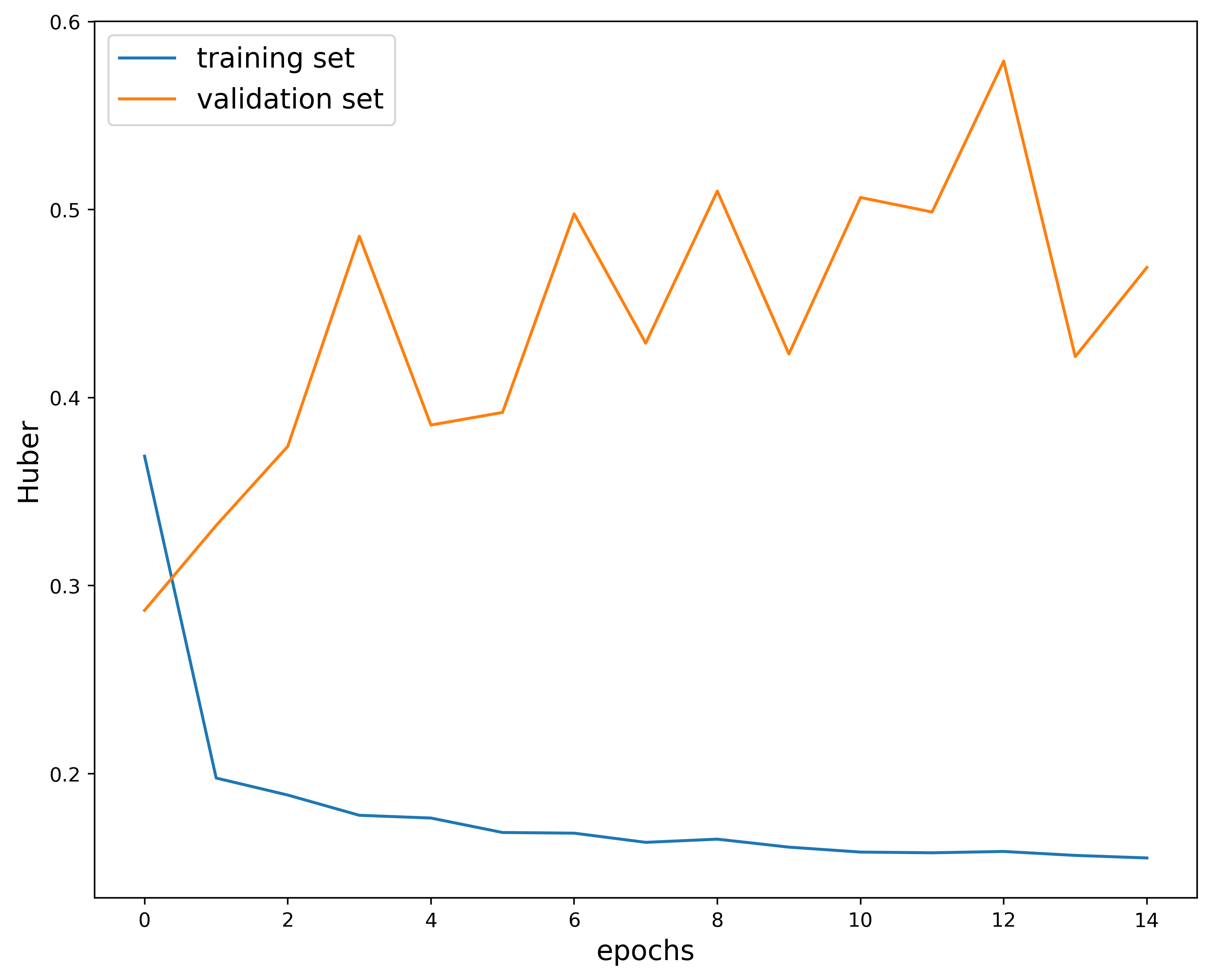
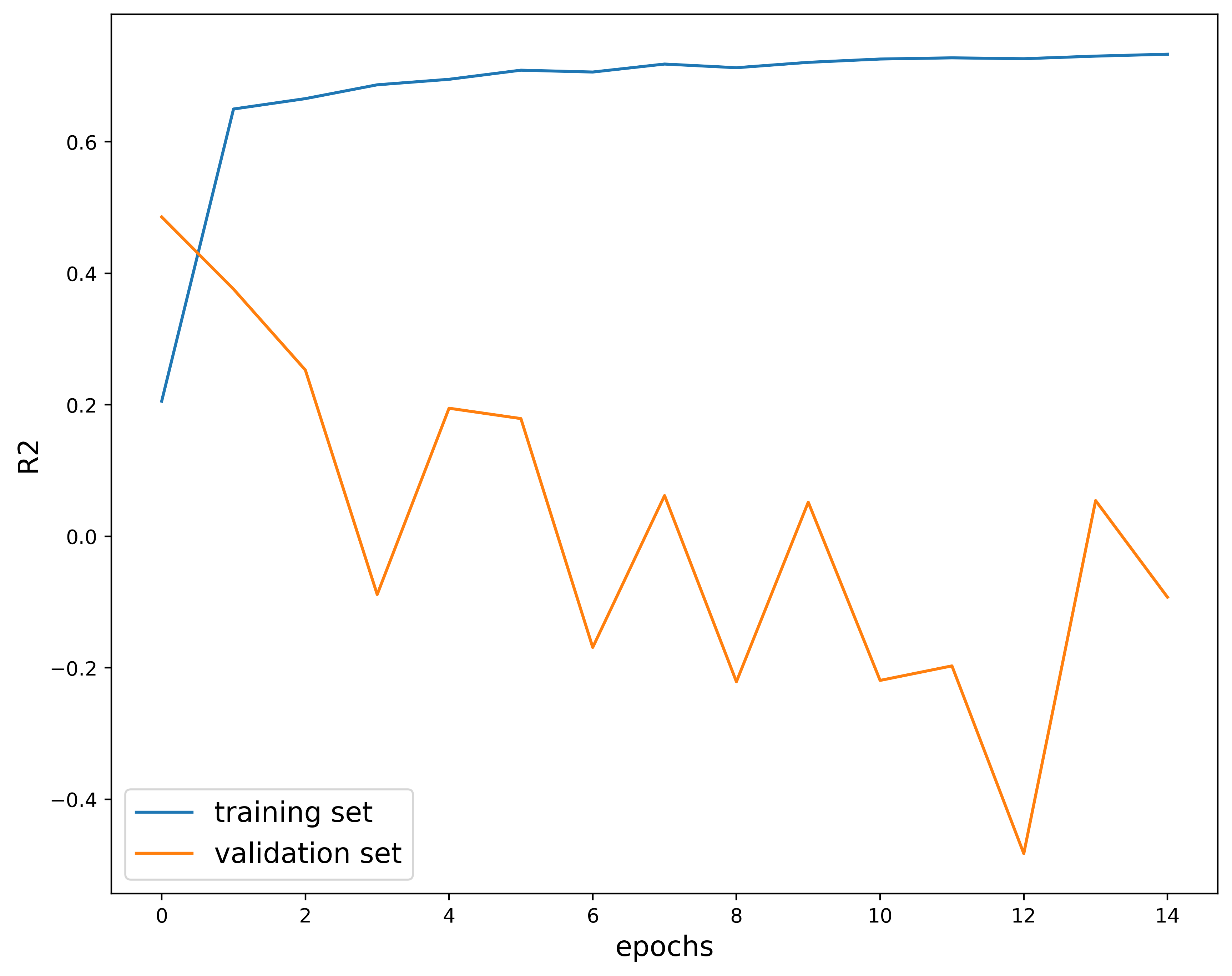
Just looking at the plots we can tell that these hyperparameters are not a good choice. While the training loss looks decent, the validation loss does not decrease as we increase the number of epochs. This implies that the model is not learning the dataset.
Second example:
params #12: (0.001, 32, 0.6)
While the loss may look good, the validation loss also crossed over the training loss. While we can just stop training early, the loss curves do not decay as nicely as the base model.
Third example:
params #20: (0.0001, 32, 0.3)
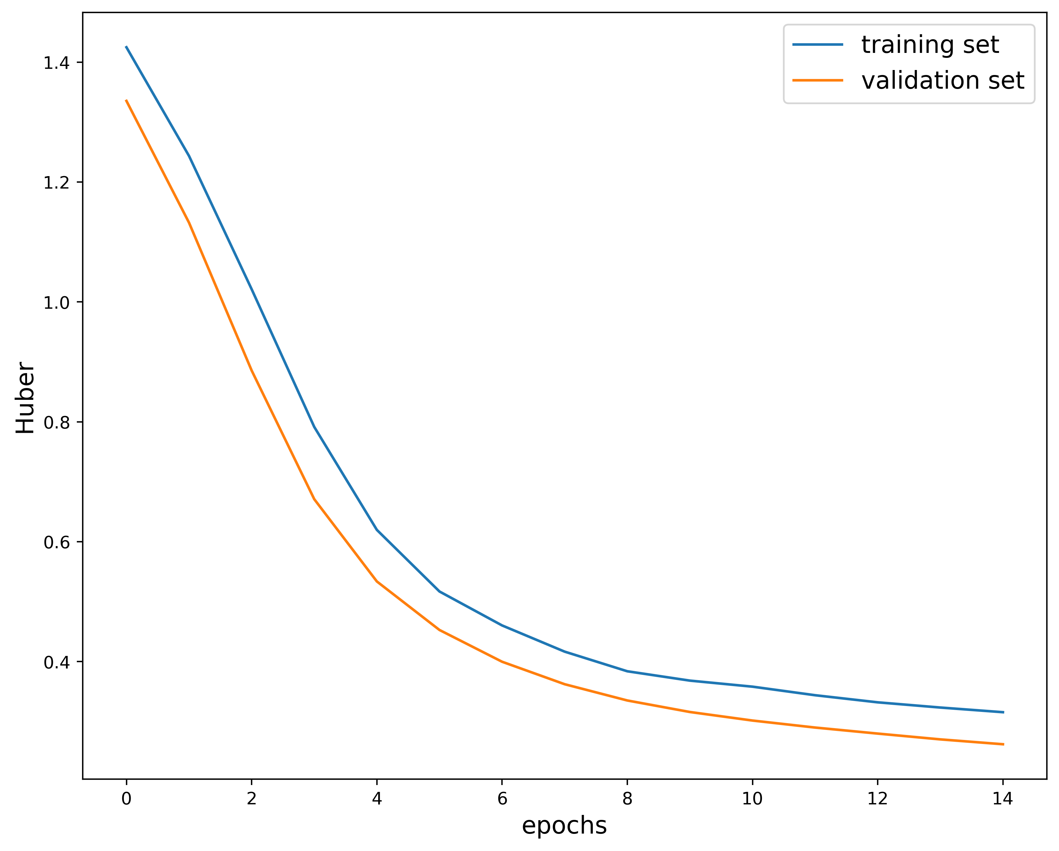
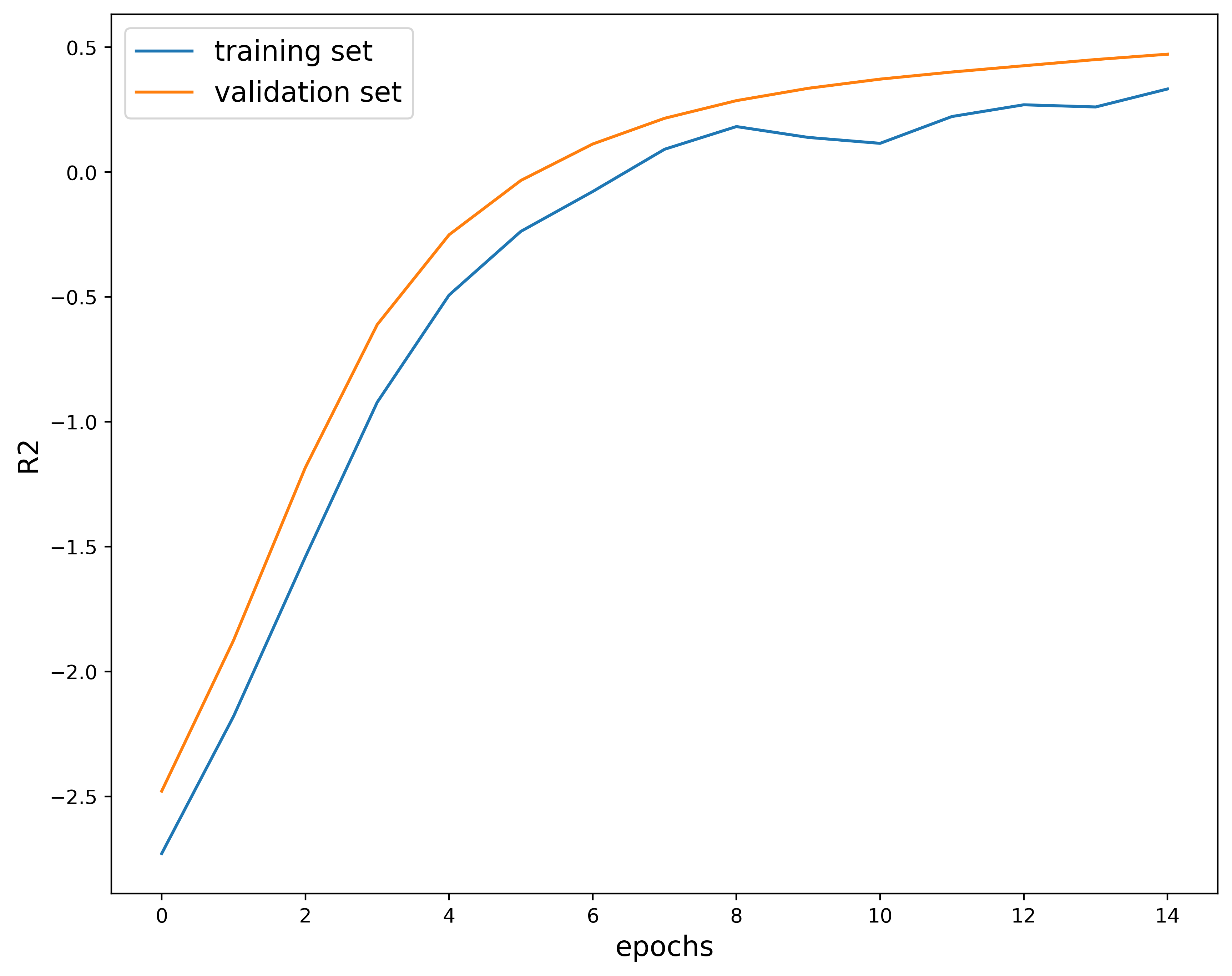
These loss curves look better than the previous two and there is no crossing of the loss. The model seems to be slowly learning over time since there is not a sharp drop in the loss. The $R^2$ score also increases and levels out nicely. These hyperparameters are a good choice. Let’s take a closer look at the metrics outputs:
Epoch 13:
New best model at epoch 13 (val_loss=0.2799)
Train - Huber: 0.3321, R2-score: 0.2695
Validation - Huber: 0.2799, R2-score: 0.4258

Epoch 14:
New best model at epoch 14 (val_loss=0.2703)
Train - Huber: 0.3234, R2-score: 0.2608
Validation - Huber: 0.2703, R2-score: 0.4506

Epoch 15:
New best model at epoch 15 (val_loss=0.2622)
Train - Huber: 0.3156, R2-score: 0.3327
Validation - Huber: 0.2622, R2-score: 0.4720

Test - Huber: 0.3395, R2-score: -10.3754
The metrics outputs seem fine, but the $R^2$ score on the test dataset is $-10.375$. Not only is it negative, but it is beyond the range we mentioned earlier in the post. If they do not perform well on the test dataset, they may not be a good choice.
Fourth example:
params #26: (0.0001, 128, 0.3)
These loss curves also look really nice. It seems that the model learns quickly at first with these hyperparamters, then does not change as much with increasing epochs. The $R^2$ score also increases and levels out similar to the third example. These hyperparameters are also a good choice. Let’s take a closer look at the metrics outputs:
Epoch 13:
New best model at epoch 13 (val_loss=0.1993)
Train - Huber: 0.2310, R2-score: 0.5754
Validation - Huber: 0.1993, R2-score: 0.6467

Epoch 14:
Train - Huber: 0.2255, R2-score: 0.5897
Validation - Huber: 0.2010, R2-score: 0.6438

Epoch 15:
Train - Huber: 0.2251, R2-score: 0.5873
Validation - Huber: 0.1999, R2-score: 0.6470

Test - Huber: 0.2179, R2-score: 0.3668
The model seems to be performing well with the test set so these hyperparameters seem to be a good choice.
At first glance, the last two examples appear to be good choices and may be better than our initial base model. If we then check how well the model performs in the test phase, we see that the third example does not perform well on the new data. On the other hand, the fourth example outputs a decent $R^2$ score and loss, so we would choose this set of hyperparameters.
We also display a table with all the results:
|         Model          | Validation loss | Test loss | Test R2-score |
| ---------------------- | --------------- | --------- | ------------- |
|       base_model       |    0.200688     | 0.213490  |   0.607139    |
| lr0.001_hdim128_do0.0  |    0.216196     | 0.610909  |   -0.554772   |
|  lr0.001_hdim32_do0.3  |    0.205734     | 0.313990  |   0.435274    |
| lr0.0001_hdim128_do0.6 |    0.215220     | 0.243275  |   -0.366992   |
| lr0.001_hdim128_do0.6  |    0.199085     | 0.375953  |   -0.558818   |
| lr0.0001_hdim32_do0.3  |    0.262168     | 0.339538  |  -10.375393   |
| lr0.0001_hdim32_do0.6  |    0.294543     | 0.387825  |  -14.893430   |
| lr0.0001_hdim128_do0.3 |    0.199262     | 0.217917  |   0.366839    |
| lr0.0001_hdim32_do0.0  |    0.236734     | 0.313647  |   -9.647883   |
|  lr0.001_hdim32_do0.0  |    0.226325     | 0.479087  |   -0.094879   |
| lr0.001_hdim128_do0.3  |    0.211276     | 0.545321  |   -0.268541   |
|  lr0.01_hdim128_do0.6  |    0.238816     | 0.413160  |   0.192252    |
|  lr0.01_hdim128_do0.0  |    0.340562     | 0.796216  |   -1.484344   |
|  lr0.01_hdim64_do0.6   |    0.263552     | 0.396611  |   0.212692    |
|  lr0.01_hdim32_do0.0   |    0.371635     | 0.866089  |   -1.596811   |
|  lr0.01_hdim128_do0.3  |    0.299062     | 0.650552  |   -0.698870   |
|  lr0.001_hdim32_do0.6  |    0.199160     | 0.269113  |   0.536666    |
|  lr0.001_hdim64_do0.6  |    0.196005     | 0.351168  |   0.295199    |
| lr0.0001_hdim64_do0.3  |    0.227803     | 0.253033  |   -0.336243   |
| lr0.0001_hdim64_do0.6  |    0.246033     | 0.315547  |   -8.151037   |
| lr0.0001_hdim128_do0.0 |    0.184923     | 0.203477  |   0.591489    |
| lr0.0001_hdim64_do0.0  |    0.210855     | 0.221721  |   0.612034    |
|  lr0.001_hdim64_do0.3  |    0.205427     | 0.478154  |   -0.110683   |
|  lr0.001_hdim64_do0.0  |    0.194936     | 0.580364  |   -0.837558   |
|  lr0.01_hdim64_do0.0   |    0.295101     | 0.704713  |   -0.920688   |
|  lr0.01_hdim32_do0.6   |    0.232968     | 0.288357  |   0.498615    |
|  lr0.01_hdim32_do0.3   |    0.286834     | 0.489060  |   -0.104738   |
|  lr0.01_hdim64_do0.3   |    0.240279     | 0.565656  |   -0.386141   |
This table shows a summary of the results of the hyperparameter tuning. The table contains the model name, the validation loss, test loss, and test $R^2$ score for the base model and all the combinations of hyperparameters.
Overall, we can use hyperparameter tuning to figure out what is the best combination of values we can use to get a well-performing model. In this post I showed the basics, but there are other hyperparameters that can be tuned, such as batch size, number of hidden layers, and optimizer momentum. In addition, one can also use techniques such as random search when working with large number of values or hyperparameter, or Bayesian optimization when evaluating the model is computationally time-consuming. When there are issues with the model, we can use gradient norm checking to get a better understanding of the behavior of the gradients across all layers and epochs. This may not always be useful, but its another tool one can use to check performance.
The code presented and plots displayed in this and the previous post can be found on my Github under the build-mlp repo.
Feel free to reach out if you have any questions about what we covered this week. I will take a break the next few weeks and come back with natural language processing examples. Stay tuned!