Linear regression: A review of projectile motion
August 16, 2025
With all the buzz surrounding AI and machine learning, it is not uncommon to hear the term ‘‘linear regression’’ being thrown around. But what is linear regression? Linear regression is a technique that can be used to model the relationship between a dependent quantity and an independent quantity. For example, the weather is a dependent quantity that depends on the time of day, which is the independent quantity. The method is called linear because it models using a linear relationship. Overall, you are trying to learn the relationship between two variables using a linear fit.
With linear regression, one can then use the independent quantities to predict the its dependent counterpart. For example, if we applied linear regression to a data composed of energies and their corresponding potential energies, we can make predictions on energies that we do not have data on.
Before that, I will do a quick review on projectile motion and show how to code the kinematic equations up in Python. Kinematics is the study of how objects move, with the focus being on quantities such as time, velocity, and position as opposed to forces. Some basics equations that describe kinematics in one-dimension are
\[\begin{aligned} x &= x_0 + v_0 t + \frac{1}{2} a t^2,\\ v &= v_0 + a t^2. \end{aligned}\]Here, $x$ is the final position, $v$ is the final velocity, $x_0$ is the initial position, $v_0$ is the initial velocity, $a$ is the acceleration, and $t$ is the time. If we want to consider motion in two dimensions, we must increase the number of equations. Now, we have
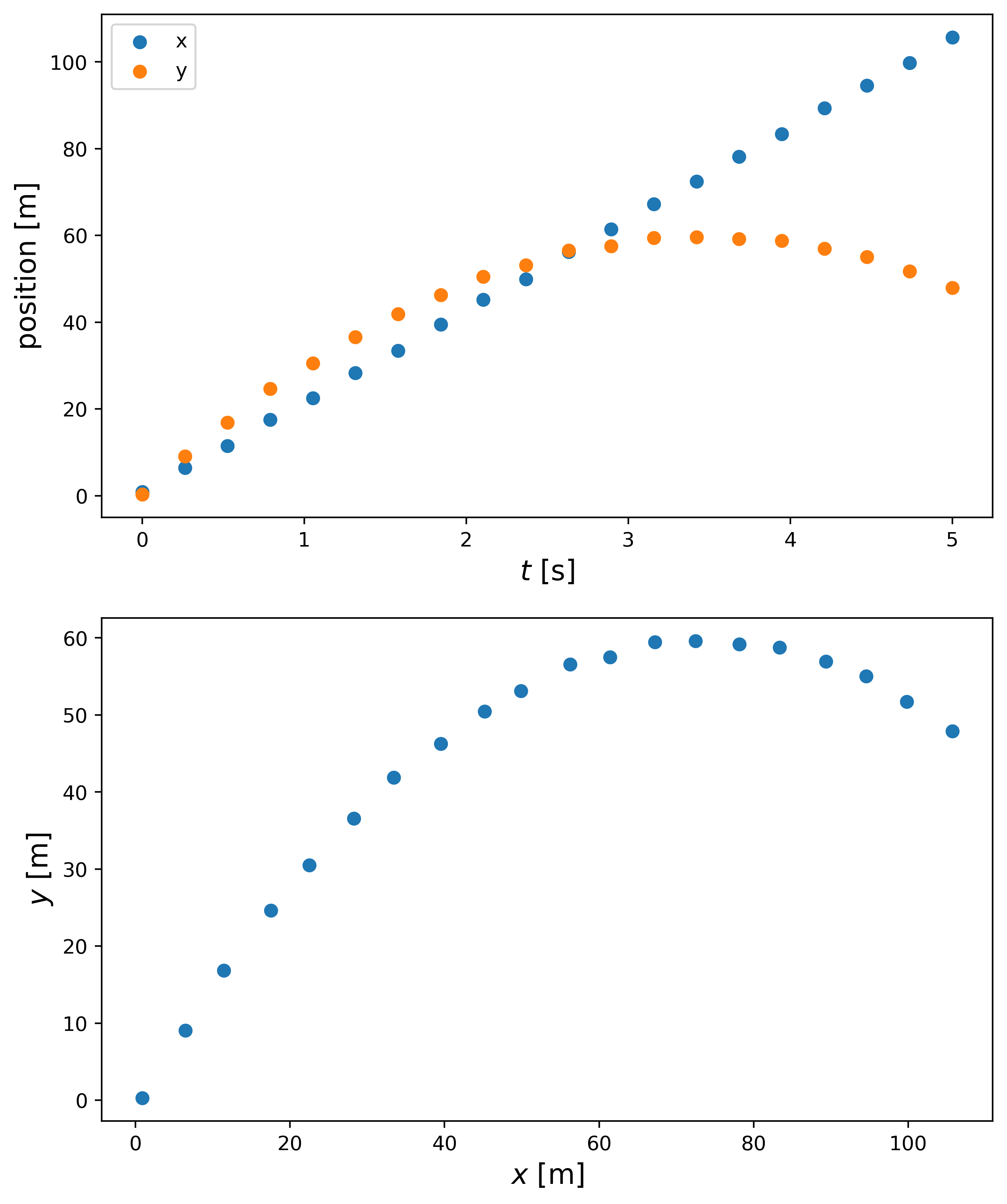
\[\begin{aligned} x &= x_0 + v_{x0} t,\\ y &= y_0 + v_{y0} t + \frac{1}{2} g t^2,\\ \\[0.1em] v_{x0} &= v_0 cos(\theta),\\ v_{y0} &= v_0 sin(\theta),\\ \\[0.1em] v_x &= v_{x0},\\ v_y &= v_{y0} + g t^2, \end{aligned}\]where now we have added equations for $x$ and $y$ independently. Here, $g$ is the acceleration due to gravity $g = -9.81 \, m/s^2$. A keen eye would notice that there is an acceleration term in the $y$ equations, but not in the $x$ equations. This is because the only acceleration present is the one due to gravity. More complicated problem can model other accelerations, but for a simple kinematics problem $y$ will only have acceleration due to gravity and $x$ will have no acceleration. Here is a graph of the equation with the accompanying Python code:
def pos_eq(p0, v0, a, t, noise=False):
    p = p0 + v0*t + 0.5*a*t**2

    if noise:
        p += tc.rand(t.shape)
    return p

noise = True

ax = tc.asarray([0])
g = tc.asarray([-9.81])

x0 = tc.asarray([0])
y0 = tc.asarray([0])
v0 = tc.asarray([40])
theta = tc.asarray([45])
v0x = v0*tc.cos(theta)
v0y = v0*tc.sin(theta)

t = tc.linspace(0, 5, 20)
x_t = pos_eq(x0, v0x, ax, t, noise)
y_t = pos_eq(y0, v0y, g, t, noise)

t_pred = tc.linspace(5.5, 8, 8).reshape(-1, 1)
x_t_pred = pos_eq(x0, v0x, ax, t_pred, noise)
y_t_pred = pos_eq(y0, v0y, g, t_pred, noise)
As we can see from the code I will be modeling an object being thrown at a $45$ degree angle with a velocity of $v_0 = 40$ m/s. The initial start point will be $x_0 = y_0 = 0$ m. The object will travel for $t = 5$ s. We also define times where the model will be trying to predict the position, $t_\text{pred}$. In order to draw comparisons between the model and the truth, we calculate what the true positions should be. We also choose to add a small amount of random Gaussian noise to the positions.
Feel free to reach out if you have any questions about what we covered this week. Next time, I will go over using Scikit-learn to apply linear regression to the projectile motion problem we just went over. Stay tuned!