Linear regression: Applying Scikit-learn to projectile motion example
August 23, 2025
Last time, we went over projectile motion and how to code the equations up in Python. In this post, I will show how to apply linear regression in Python using Scikit-learn’s LinearRegression.
The example we will be working with is a standard two-dimensional kinematics problem. We will have data for only the first two-thirds of the path traveled and we will use linear regression to predict positions past what we have. I will exclusively work with PyTorch tensors and only convert to numpy arrays when needed.
We will be using the class sklearn.linear_model.LinearRegression. The following code applies the linear regression algorithm to our data using Scikit-learn:
def generate_rand_numbers(a, b, N):
    return (b - a) * tc.rand(N) + a

a, b = t[0], t[-1]
t_rand = generate_rand_numbers(a, b, t.shape[0]).reshape(-1, 1)
x = pos_eq(x0, v0x, ax, t_rand, True)
y = pos_eq(y0, v0y, ay, t_rand, True)

t_poly = tc.concat([t_rand, t_rand**2], dim=-1)
t_poly_pred = tc.cat([t_pred, t_pred**2], dim=1)

model = LinearRegression()
model.fit(t_rand, x)
x_skl = np.squeeze(model.predict(t_rand))
x_skl_pred = np.squeeze(model.predict(t_pred))

model = LinearRegression()
model.fit(t_poly, y)
y_skl = np.squeeze(model.predict(t_poly))
y_skl_pred = np.squeeze(model.predict(t_poly_pred))
The process is as follows:
- Generate random times within some interval give by the start and end time.
- Calculate the position values of of random times for both $x$ and $y$.
- Initialize the model.
- Fit the model using the random times and their associated positions.
- Use the model to predict the positions at new, unseen times.
One thing to note:
For the $y$ position, we need to reshape the input variables $t_\text{rand}$ and $t_\text{pred}$ as shown by $t_\text{poly}$ and $t_\text{poly_pred}$. The reason is that the equations are not linear, but the class expects to perform a linear regression. The key here is that although the equations are not linear in $t$, they are in fact linear in the parameters that the model is trying to learn as shown below:
where the parameters the model is trying to fit are $w_1$, $w_2$, $w_3$, and $b$.
Here are the results of the linear regression:
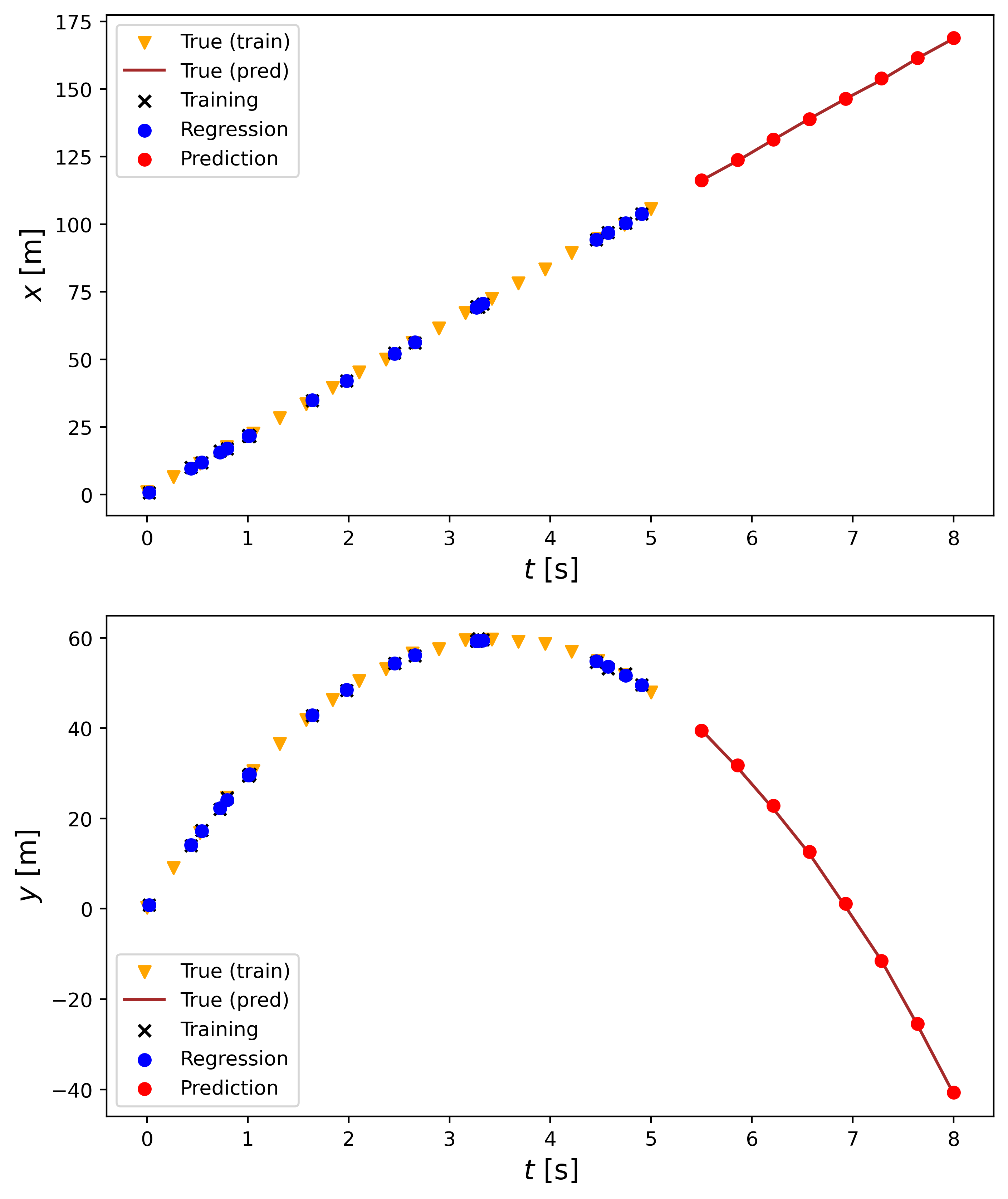
The upper plot shows the linear regression process for the $x$ position and the lower one for the $y$ position. From the legend, we see that the true values that were used to pick the random times are given in yellow triangles, the true values for the times we are trying to predict are given by the brown line, the training values ($t_\text{rand}$) are given by the black x, the predicted position of the $t_\text{rand}$ values are given by blue dots, and the prediction for the new times are given by red dots. As can be seen, the model does a good job of predicting the positions for the times we do not have data for since the predictions match up with the truth.
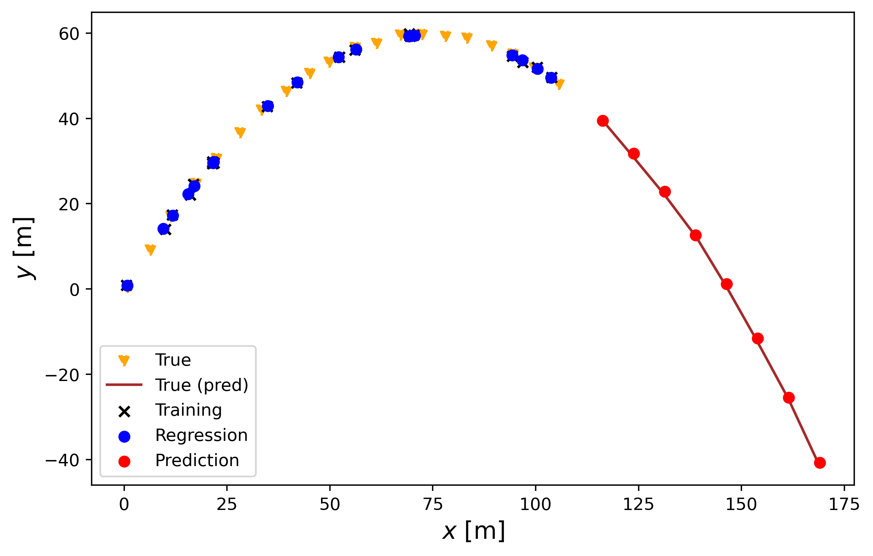
The following plot shows how the trajectory would look to a person watching the object being thrown.
Here are the absolute errors:
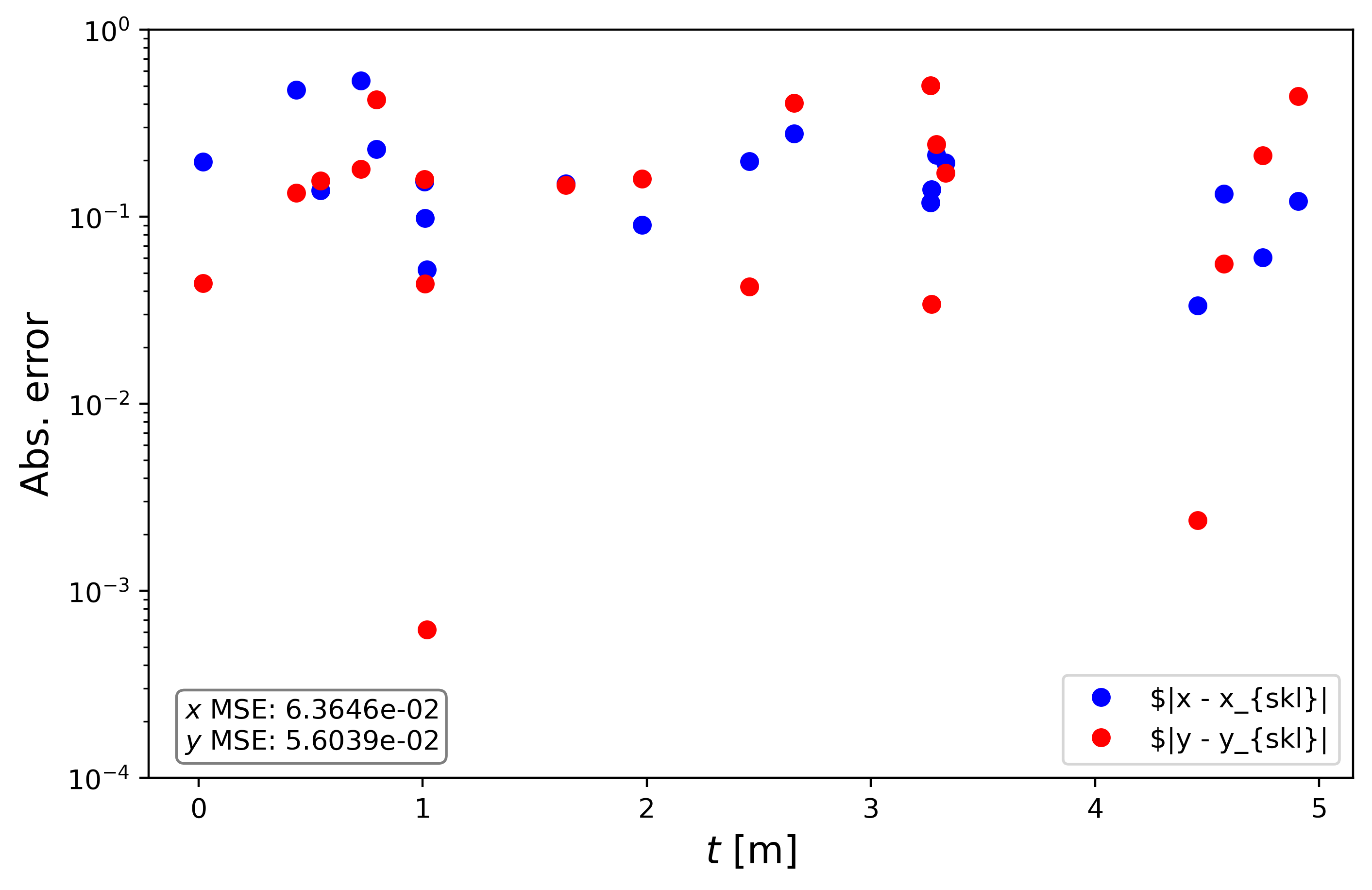
The overall mean square error (MSE) is on the order of $10^{-2}$, which in this case is good enough since we are dealing with meters. The reason as to why the MSE is not smaller is because of the noise we added to the data. In this case, the noise is the most dominant error, which prevents the model from achieving a more accurate prediction.
Feel free to reach out if you have any questions about what we covered this week. Next time, I will go over how to perform linear regression using PyTorch. Stay tuned!