Linear regression: Applying PyTorch to projectile motion example

August 31, 2025

Last time, we went over how to apply linear regression to a problem using Scikit-learn. I showed the process and the results of Scikit-learn’s LinearRegression. In this post, I will show how to apply linear regression in Python using PyTorch. We will be using the same projectile motion example as before.

We will be using the class torch.nn.Linear. Before we build the linear layer we need to normalize our data. It is standard practice to normalize the data whenever you use a model that performs backpropagation. This has various positive effects such as:

1. Improved learning
   
   • If the inputs are too large, the gradient descent will bounce around too much, which makes it difficult for the model to learn.
     
   • If the inputs are too small, the gradient descent will move too slow, which makes learning very slow.
     
2. Avoid exploding gradients
   
   • If the inputs are too large, this can lead to large gradients in backpropagation, which will hinder learning. This is known as the exploding gradient problem.
     
   • If the inputs are too small, this can lead to small gradients in backpropagation, which will also hinder learning. This is known as the vanishing gradient problem.
     
3. Faster convergence
   
   • By normalizing the input data, one creates a more well-conditioned loss surface, which allows the optimizer to take more efficient steps.
     
   • Leads to a faster and more efficient training stage.

Here is the process of normalizing the data:

def gaussian_norm(x, std, mean):
    return (x - mean) / std

def inverse_gaussian_norm(x, std, mean):
    return x * std + mean

t_std, t_mean = tc.std(t_rand), tc.mean(t_rand)
x_std, x_mean = tc.std(x), tc.mean(x)
y_std, y_mean = tc.std(y), tc.mean(y)

t_norm = gaussian_norm(t_rand, t_std, t_mean)
x_norm = gaussian_norm(x, x_std, x_mean)
y_norm = gaussian_norm(y, y_std, y_mean)

Note:
Since we are normalizing the inputs, the outputs will also be normalized. This means that after we make a prediction, we have to “unnormalize” the result. The function I use to do this is inverse_gaussian_norm().

The following code is the class used to apply the linear layer to our data:

class BuildLinearLayer():
    def __init__(self, num_features, lr, bias=True):
        self.model = nn.Linear(in_features=num_features[0], 
                               out_features=num_features[1], 
                               bias=bias)
        self.loss_fn = nn.MSELoss()
        self.optimizer = tc.optim.SGD(self.model.parameters(), lr=lr)

    def concat_nonlinear(self, X):
        return tc.cat([X, X**2], dim=1)
        
    def train(self, X, y, epochs, atol=1e-8):
        model = self.model
        loss_fn = self.loss_fn
        optimizer = self.optimizer
        
        prev_loss = 0

        if model.in_features > 1:
            X_feat = self.concat_nonlinear(X)
        else:
            X_feat = X
        
        for i, epoch_i in enumerate(range(epochs)):
            y_pred = model(X_feat)
            loss = loss_fn(y_pred, y)
            
            optimizer.zero_grad()
            loss.backward()
            optimizer.step()
        
            if (i + 1) % 100 == 0:
                print(f'epoch = {i + 1}, loss = {loss}')
                plot_true_vs_pred(X, y, tc.squeeze(y_pred).detach())
        
            if abs(prev_loss - loss) < atol:
                print('Training done')
                print(f'Epoch = {i + 1}, loss = {loss}')
                print(f'Residual: {abs(prev_loss - loss)} < {atol}')
                plot_true_vs_pred(X, y, tc.squeeze(y_pred).detach())
                break
    
            prev_loss = loss

        return None
            
    def predict(self, X):
        model = self.model

        if model.in_features > 1:
            X_feat = self.concat_nonlinear(X)
        else:
            X_feat = X
        
        with tc.no_grad():                
            y = model(X_feat)
            
        return tc.squeeze(y.detach())

The linear layer is initialized in the constructor. We pass in the number of inputs, number of outputs, and whether or not it has a bias. In this case, adding a bias is ideal since we are trying to model a linear equation. We choose mean square error as our loss function and Stochastic Gradient Descent (SGD) as our optimizer with a learning rate that we initialize.

The train function is where the model will be trained. First, we check the input size. Since the equations for $x$ and $y$ differ in powers of $t^2$, the input size will be different when initializing the linear layer (more on this later). If the input size is greater than $1$, we call concat_nonlinear() on the data to reshape the input variables (see the previous post).

The training process is as follows:

1. Make a prediction using the input data.
   
2. Pass that prediction and the true values into the loss function.
   
3. Zero the gradients to get rid of older gradients.
   
4. Propagate the loss backwards through the model (backpropagation).
   
5. Step the optimizer.

This is the basic process used for training the linear model. The rest of what’s in the loop is not necessarily needed, but it is nice to have. The first if statement is used to plot the predictions at set intervals to get an idea as to how the model is training as we iternate through the number of epochs. The second if statement is used to stop the training process once the model is prediction at some absolute error below a threshold. We can choose to let the model train for all epochs, but this is not really necessary if the model’s prediction is within an acceptable tolerance.

The predict function is used to make predictions on a given set of inputs. It’s important that tc.no_grad() is used because you do not need the model to keep track of the gradients since there will be no backpropagation. In this specific example, it is not an issue if the gradients are calculated, but when you get to more complex models that take in more data and need to tune more parameters (hence more gradients), calculating the gradients when not necessary can take up memory and computation time that may be needed for training or parameter tuning.

The following code calls the class:

epochs = 2000
lr = 0.01

# Linear layer for x
my_ll = BuildLinearLayer([1, 1], lr)
my_ll.train(t_norm, x_norm, epochs)
x_ll_norm = my_ll.predict(t_norm)
x_ll = inverse_gaussian_norm(x_ll_norm, x_std, x_mean)

# Prediction for x
t_pred_norm = gaussian_norm(t_pred, t_std, t_mean)
x_ll_pred_norm = my_ll.predict(t_pred_norm)
x_ll_pred = inverse_gaussian_norm(x_ll_pred_norm, x_std, x_mean)

# Linear layer for y
my_ll = BuildLinearLayer([2, 1], lr)
my_ll.train(t_norm, y_norm, epochs)
y_ll_norm = my_ll.predict(t_norm)
y_ll = inverse_gaussian_norm(y_ll_norm, y_std, y_mean)

# Prediction for y
t_pred_norm = gaussian_norm(t_pred, t_std, t_mean)
y_ll_pred_norm = my_ll.predict(t_pred_norm)
y_ll_pred = inverse_gaussian_norm(y_ll_pred_norm, y_std, y_mean)

We choose the number of epochs to be $2000$ and set the learning rate for the optimizer at $10^{-2}$. We will be training two linear layers, one for $x$ in terms of $t$ and one for $y$ in terms of $t$. As can be seen for $y$, we are setting the number of features going into the model to $\text{in_feature} = 2$ since we have $x$ and $x^2$ and both will need weights, and setting the number of features going out of the model to $\text{out_feature} = 1$ since only one $y$ value will be predicted per $x$ and $x^2$. In contrast, $x$ only needs $\text{in_feature} = 1$ since it has no $x^2$ term. As previously mentioned, we need to unnormalize the predictions since the output will be normalized. This process is done for both the $x$ and $y$ prediction.

Here are the results of the linear layer:

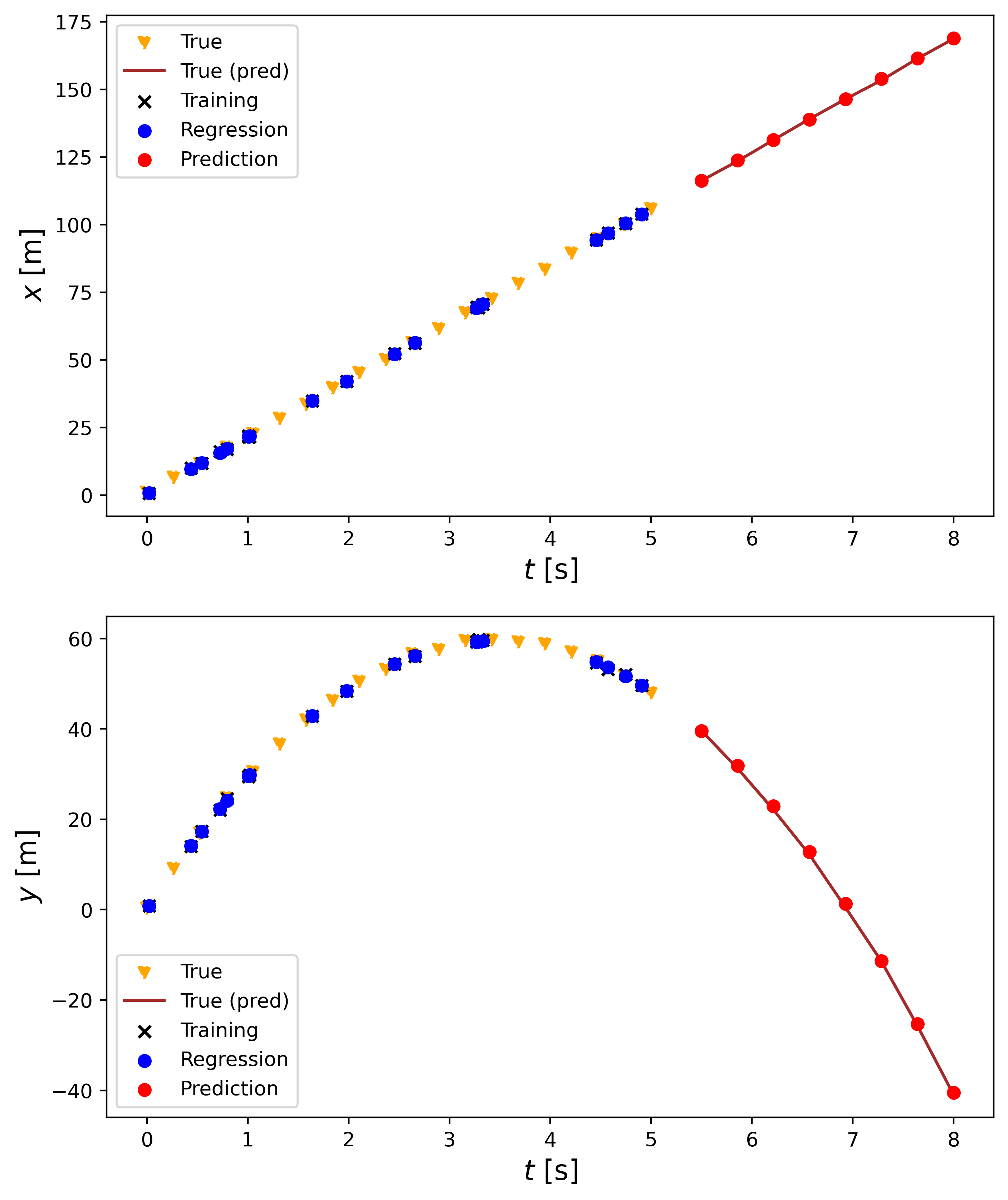
The upper plot shows the linear regression process for the $x$ position and the lower onefor the $y$ position. From the legend, we see that the true values that were used to pick the random times are given in yellow triangles, the true values for the times we are trying to predict are given by the brown line, the training values ($t_\text{rand}$) are given by the black x, the predicted position of the $t_\text{rand}$ values are given by blue dots, and the prediction for the new times are given by red dots. Similar to Scikit-learn’s LinearRegression(), the model does a good job of predicting the positions for the times we do not have data for since the predictions match up with the truth.

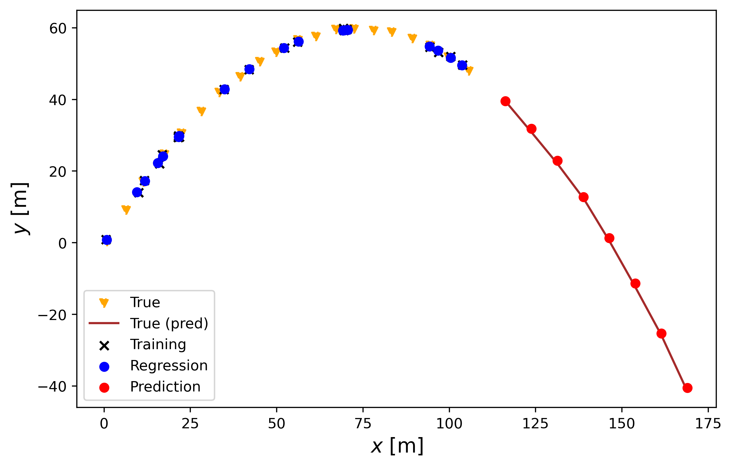
The following plot shows how the trajectory would look to a person watching the object being thrown.

Here are the absolute errors:

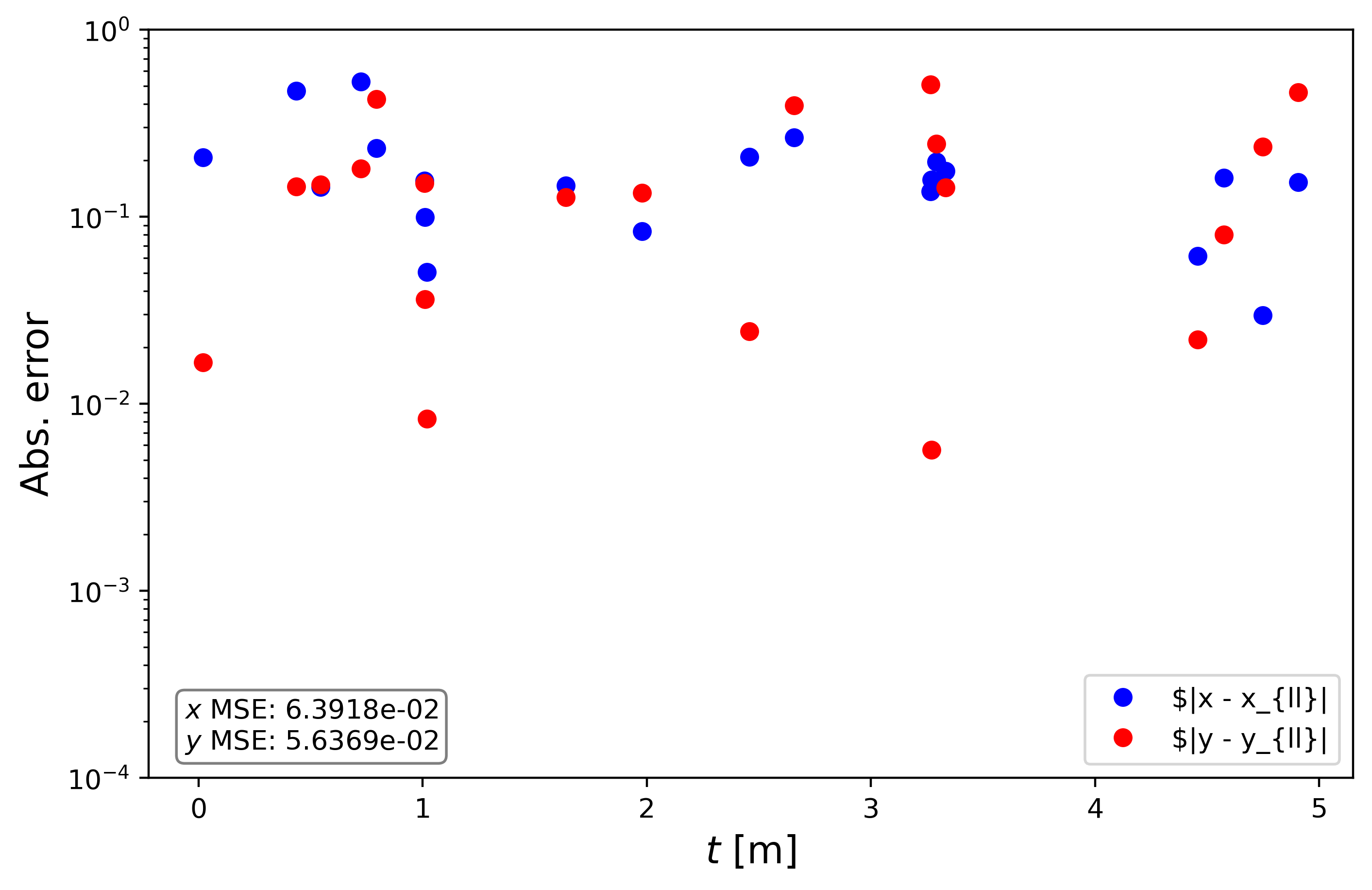
The overall mean square error (MSE) is on the order of $10^{-2}$, the same as LinearRegression() with the same conclusion. Lets compare the errors between Scikit-learn and PyTorch:

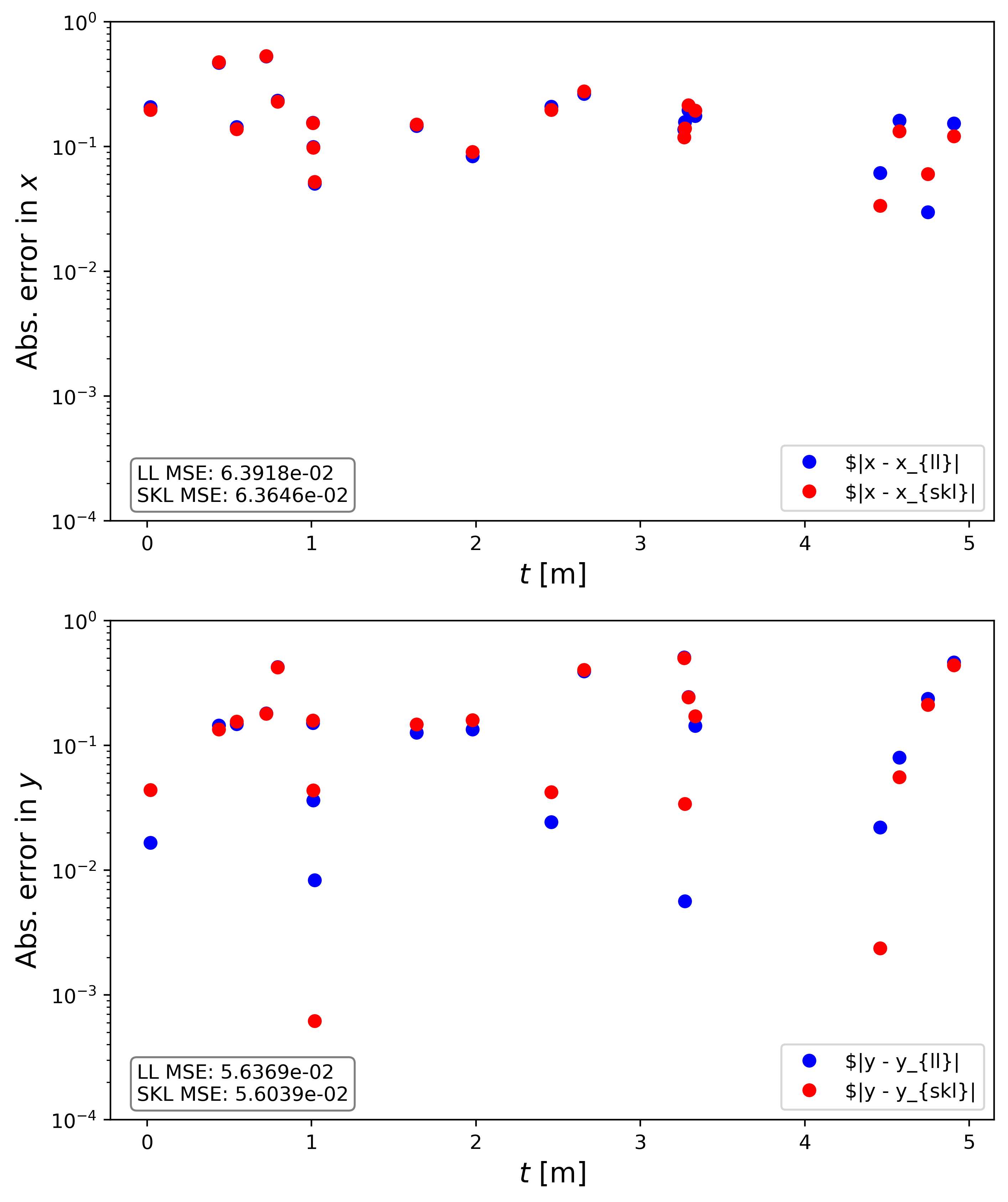
The upper plot shows the absolute error for both methods in $x$ and the bottom in $y$. The MSE is given in the bottom left corner of each plot, where LL is the linear layer and SKL is the scikit-learn implementation. We see that they are pretty much the same. In some cases LinearRegression() performs slightly better, in other cases nn.Linear() performs better. Overall, as previously mentioned, we are limited by the noise in the data so neither model can prediction at an accuracy below the noise floor.

The lingering question is probably, “Which should I use: Scikit-learn or PyTorch?” Let’s go over the differences between Scikit-learn’s LinearRegression and PyTorch’s Linear:

Scikit-learn pros:

1. Easy to use
   
   • From last week’s blog you can see that using LinearRegression() is very straightforward. All you need to do to train the model is call LinearRegression().fit(t, y).
     
2. Efficient, well-known solvers
   
   • The solvers used in LinearRegression() are efficient. Some examples are singular value decomposition (SVD) and Ordinary Least Squares (OLS).
     
3. Built-in tools
   
   • Scikit-learn has a lot of useful libraries that ready to use, such as preprocessing functions and cross-validation.

Scikit-learn cons:

1. Doesn’t generalize well
   
   • Most of the Scikit-learn implementations are meant for classical machine learning problems. If you want something you can customize and have more control over, Scikit-learn may not be what you need.
     
2. No GPU support
   
   • The models can only be trained on the CPU. While this is fine for small problems, training will become a huge bottleneck for bigger, more complicated problems you train on the CPU.
3. Scaling issues
   
   • Does not scale well for large data sets and deep learning architectures.

PyTorch pros:

1. Flexibility
   
   • You have much better control over your models and can include custom loss functions and optimization schemes. PyTorch is like a sandbox where you can try to figure out what combinations of loss functions, layers, and optimizers produce the best model for your dataset.
2. GPU support
   
   • Can push training to the GPU using CUDA.
3. No scaling issues
   
   • No issue with scaling to large data sets or more advanced deep learning architectures such as neural networks.

PyTorch cons:

1. Takes more effort
   
   • As can be seen from the code, setting up training using PyTorch is more work than with Scikit-learn. One must specify the optimizer, the loss function, the layers, etc.
2. Can be overkill for simple problems
   
   • As mentioned in the previous bulletpoint, the setup is more complicated than with Scikit-learn. This may not be ideal for simple problems.
3. Not as many built-in tools
   
   • There are no built-in libraries that take care of tasks needed for machine learning problems, such as preprocessing, metrics, etc.

Overall, Scikit-learn is a solid choice if one is solving classic problems with small to medium datasets and need an out-of-the-box solution. Additionally, it is great for learning the basics of machine learning. On the other hand, PyTorch is great for deep learning problems with large datasets since training can be moved over to the GPU and because of the allowed customization in building your model.

The code presented and plots displayed in the Linear Regression posts can be found on my Github under the linear-regression repo.

Feel free to reach out if you have any questions about what we covered this week. Next time, I will teach you about convolutional neural networks (CNNs). Stay tuned!

⬅ Back to Home