Convolutional neural networks: MNIST dataset
September 07, 2025
Today we will learn about convolutional neural networks (CNNs). A CNN is a neural network designed to process grid-like data, such as images. It works by applying a convolution, filters (usually small $n \times n$ matrices) that slide over the data to extract useful features, across the 2D grid to detect features such as edges and shapes. We can apply these neural networks to images so that the network can learn how to classify images. In this post, we will construct a CNN and apply it to preprocessed images known as the MNIST dataset.
What is MNIST?
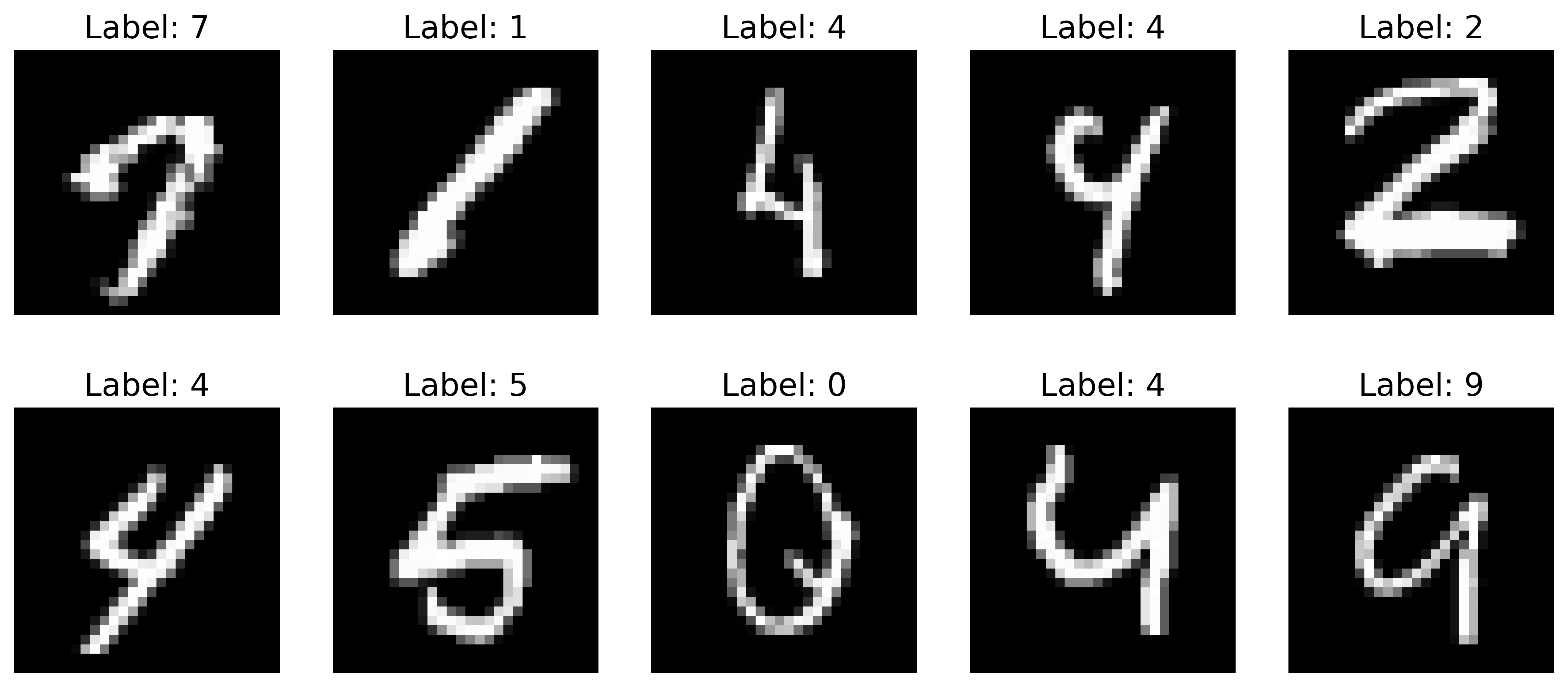
MNIST stands for Modified National Institute of Standards and Technology, which is the institute that first created this dataset. The dataset is composed of thousands of grayscale images of handwritten numbers from $0$ to $9$ (ten categories). It is a very popular dataset used when one is first learning about CNNs since it is simple and easy to understand. The documentation for the function that we will be using to load the MNIST dataset can be found here. Here is a plot of a small subset of the dataset:
Let’s jump into creating the model.
First, we must import the data. I used the MNIST dataset provided by Scikit-learn:
from sklearn.datasets import fetch_openml

mnist = fetch_openml('mnist_784', version=1)
X = mnist.data.values.astype('float32') / 255.0
y = mnist.target.astype('int64')
The $255$ is used to normalize the dataset between $0$ and $1$. This comes from the fact that a single byte ($8$ bits) can store $2^8=256$ different values. For images, this means there are $256$ different shades per each color channel. Note that we divide by $255$ instead of $256$ because Python starts at $0$ instead of $1$.
We must now split this dataset into a training set, validation set, and testing set. The training set will be used to train the model, the validation set is used to see how well the model has generalized at each epoch, and the testing set is used at the end to see how well the fully trained model can predict on a new dataset. While not everyone uses a validation set, it is good to have since it tells us how well our model is generalizing after each epoch. This will tell us at a glance whether or not our model is overfitting as it learns more.
# Train/validation split
X_train, X_val, y_train, y_val = train_test_split(X, y, test_size=0.1, random_state=42)
X_train, X_test, y_train, y_test = train_test_split(X_train, y_train, test_size=0.1, random_state=42)
The function train_test_split() only splits data into two sets so we pass in the data twice to get all three datasets. The overall split is going to be $80\%$ training set, $10\%$ validation set, and $10\%$ testing set. We initialize the random_state so that the results are reproducible.
We also have to convert to PyTorch tensors and reshape the $X$ datasets so that the CNN can accept the data. The input expected for CNNs are $(N, C, H, W)$ where $N$ is batch size (number of images in a batch), $C$ is number of channels (for grayscale this is $1$), $H$ is the height of the image and $W$ the width. Our reshape will put the data into this format. This looks like so:
# # Convert to PyTorch tensors
X_train = tc.tensor(X_train).view(-1, 1, 28, 28)
y_train = tc.tensor(y_train.values)
X_val = tc.tensor(X_val).view(-1, 1, 28, 28)
y_val = tc.tensor(y_val.values)
X_test = tc.tensor(X_test).view(-1, 1, 28, 28)
y_test = tc.tensor(y_test.values)

# # DataLoaders
train_loader = DataLoader(TensorDataset(X_train, y_train), batch_size=64, shuffle=True)
val_loader = DataLoader(TensorDataset(X_val, y_val), batch_size=64)
test_loader = DataLoader(TensorDataset(X_test, y_test), batch_size=64)
The last step above is to set up the data loaders. First, TensorDataset() is a function that pairs the features $X$ with the labels $y$ in a tuple. The function DataLoader() then provides an iterator that iterates over minibatches of the dataset with the batch size, in this case, being $64$. We also shuffle the training data so that the model doesn’t learn the ordering and can generalize better.
Now that we have taken care of the dataset, let’s move on to the actual CNN:
class SimpleCNN(nn.Module):
    def __init__(self):
        super().__init__()
        self.conv = nn.Sequential(
            nn.Conv2d(1, 32, 3, padding=1),
            nn.ReLU(),
            nn.MaxPool2d(2),
            nn.Conv2d(32, 64, 3, padding=1),
            nn.ReLU(),
            nn.MaxPool2d(2)
        )
        self.fc = nn.Sequential(
            nn.Flatten(),
            nn.Linear(64*7*7, 128),
            nn.ReLU(),
            nn.Linear(128, 10)
        )
    def forward(self, x):
        x = self.conv(x)
        return self.fc(x)
Let’s unpack the class. First, we pass in nn.Module as an argument into the class and write super().__init__() in the constructor. This is called inheritance and ensures that all the functions normally available in the parent class nn.Module are also available in the child class, which is our define_CNN() class. In the constructor you will see nn.Sequential(), which is a container module that lets you build neural networks by stacking layers and activation functions sequentially. This container module is used in two different places, to define the CNN self.conv and the multi-layer perception (MLP) self.fc. The reason we define both a CNN and a MLP is because the CNN’s sole focus is to learn the features, while the MLP is supposed to take those features and map them to a final output (category). In this case, the CNN is known as the backbone and the MLP as the neck.
You may ask, “Why separate them?” Here are some reasons why we may want to build a model with a separate backbone and head:
- Modularity:
- You can change the convolutional part without touching the fully connected layers, or vice versa.
- Example: Add more convolutional layers, or replace
self.fcwith a different classifier.
- You can change the convolutional part without touching the fully connected layers, or vice versa.
- Conceptual clarity:
self.conv–> extract patternsself.fc–> decide which class based on patterns
- Industry standard:
- Most CNNs follow this “feature extractor + classifier” design, which makes it easier to swap backbones or use pretrained models.
Let’s look at the model and break down each layer:
The convolutional neural network:
nn.Conv2d(1, 32, 3, padding=1)
- This is a two-dimensional convolutional layer with $1$ input channel, $32$ output channels (learning $32$ features), and a convolutional kernel size of $3$. Finally, we zero pad with size $1$ to keep the spatial size of the image the same as the input since the function defaults to stride=$1$.
- This is a two-dimensional convolutional layer with $1$ input channel, $32$ output channels (learning $32$ features), and a convolutional kernel size of $3$. Finally, we zero pad with size $1$ to keep the spatial size of the image the same as the input since the function defaults to stride=$1$.
nn.ReLU()
- This is a Rectified Linear Unit activation function. It is defined as $\text{ReLU}(x) = \text{max}(0, x)$. Essentially, it zeros out the negative values while introducing non-linearity. This type of activation function is simple and fast to use compared to others such as $\text{tanh}(x)$ or sigmoid.
- This is a Rectified Linear Unit activation function. It is defined as $\text{ReLU}(x) = \text{max}(0, x)$. Essentially, it zeros out the negative values while introducing non-linearity. This type of activation function is simple and fast to use compared to others such as $\text{tanh}(x)$ or sigmoid.
nn.MaxPool2d(2)
- This is a two-dimensional max pooling layer meant to reduce spatial dimensions while keeping important information. In this case, $2$ denotes that a $2 \times 2$ kernel is used. The max pooling layer will then take a $2 \times 2$ window and slide it over the feature map, taking the maximum value within the window and assigning it to the corresponding location in the output.
nn.Conv2d(32, 64, 3, padding=1)
- This convolutional layer now has $32$ input channels, $64$ output channels, meaning it is meant to learn more finer details than the previous one since the outputs channels have now increased.
- This convolutional layer now has $32$ input channels, $64$ output channels, meaning it is meant to learn more finer details than the previous one since the outputs channels have now increased.
nn.ReLU()
- Same as before.
- Same as before.
nn.MaxPool2d(2)
- Same as before.
- Same as before.
The multi-layer perceptron:
nn.Flatten()
- This is used to flatten the input tensor. The output of the CNN is a four-dimensional tensor. Since the input to the MLP is the output of the CNN, the tensor has to be flatten.
- This is used to flatten the input tensor. The output of the CNN is a four-dimensional tensor. Since the input to the MLP is the output of the CNN, the tensor has to be flatten.
nn.Linear(64*7*7, 128)
- This is a fully connected linear layer with input size $64*7*7$ (output of CNN) and output size of $128$ neurons.
- This is a fully connected linear layer with input size $64*7*7$ (output of CNN) and output size of $128$ neurons.
nn.ReLU()
- Same as before.
- Same as before.
nn.Linear(128, 10)
- This is another fully connected linear layer, but now the input size is $128$ and the output size is $10$, which matches how many categories we have ($0$-$9$).
- This is another fully connected linear layer, but now the input size is $128$ and the output size is $10$, which matches how many categories we have ($0$-$9$).
The last part of the class is the function forward() that calls the CNN, then passes the output of the CNN to the MLP so that the features can be mapped to a category.
Now, let’s see how the model is trained. First, we need to initialize the CNN, the optimizer, and the loss function:
cnn = SimpleCNN()
optimizer = optim.AdamW(cnn.parameters(), lr=0.001)
loss_fn = nn.CrossEntropyLoss()
In this case, we will use the optimizer optim.AdamW() with an initial learning rate of $0.001$. This optimizer is a popular choice since it takes the fast convergence of Adam (another optimizer) and the generalization properties of SGD (optimizer we used last week) with weight decay. For more information on this optimizer see here. The loss function we will be using is cross-entropy loss. This loss function measures the difference between two probability distributions and is widely used for classification problems. For more information on this loss function see here.
The training will look like the following:
for epoch in range(3):
    cnn.train()
    correct, total = 0, 0
    # Trains over the training set
    for X, y in train_loader:
        optimizer.zero_grad()
        output = cnn(X)
        loss = loss_fn(output, y)
        loss.backward()
        optimizer.step()

        preds = tc.softmax(output, dim=0).argmax(1)
        correct += (preds == y).sum().item()
        total += y.size(0)
    train_acc = correct / total

    # Evaluates over the validation set
    cnn.eval() # put model in evaluation mode
    correct, total = 0, 0
    with tc.no_grad(): # no gradient tracking during evaluation
        for X, y in val_loader:
            output = cnn(X) # forward pass
            preds = tc.softmax(output, dim=0).argmax(1)
            correct += (preds == y).sum().item()
            total += y.size(0)
    val_acc = correct / total

    print(f"Epoch {epoch + 1},
            Train Accuracy: {train_acc:.8f},
            Validation Accuracy: {val_acc:.8f}")
I won’t go over all the details since some of this code is present in last week’s post, so I will only go over the new additions. In the training portion, we now implement tc.softmax() on the outputs, which converts the output prediction to probabilities that overall sum to $1$. The method .argmax(1) finds the index of the maximum value of each row. In essence, we are picking out the prediction that has the highest probability of matching up to the true target. The next line calculates how many of our predictions are actually correct, while the line after find the total number of targets that the model is supposed to predict. With these values, we can calculate a percentage of correct predictions (given by train_acc).
Like I previously mentioned, we use a validation set to determine how well our model generalizes between epochs. The next part of the loop does exactly this. We first put the model in evaluation mode using .eval(). While in evalulation mode, the weights of the model are not changed with the new data and processes like dropout are deactivated. The rest of the loop is identical to the training portion, which is just calculating the percentage of correct predictions (given by val_acc) with the validation set. After both calculation, we print out the current epoch and the accuracies. The model is trained and the validation set accuracy computed for a total of three epochs. Once done training, our model is now full trained and ready to go.
The next step is to see how the fully trained model generalizes with unseen data. We will use the same method of calculating the validation accuracy with the test data since the point is to see how well the model generalizes to unknown data. An example of what the print statement output looks like is the following:
Epoch 1, Train Accuracy: 0.88814815, Validation Accuracy: 0.94385714
Epoch 2, Train Accuracy: 0.95839506, Validation Accuracy: 0.96385714
Epoch 3, Train Accuracy: 0.97007055, Validation Accuracy: 0.96928571
Test Accuracy: 0.97190476
These numbers will change when the training is reran since we are not seeding the random numbers in PyTorch.
We have now fully trained a model composed of a CNN for feature learning and a MLP for learning the mapping between the data and the targets. We also included an evaluation over a validation set to check how well the model is generalizing to unknown data as it is being trained, and an evaluation over a test set to check how well the full trained model performs on unseen data. Overall, the model seems to be very accurate with a test accuracy of $\approx 97 \%$. That being said, there is still $\approx 3 \%$ of the test data that is not being categorized correctly. Let’s see a subset of these predictions to try to understand what is going on.
misclassified_images = []
misclassified_preds = []
true_labels = []

cnn.eval()
with tc.no_grad():
    for X, y in test_loader:
        output = cnn(X)
        preds = tc.softmax(output, dim=0).argmax(1)
        mismatches = preds != y

        if mismatches.any():
            misclassified_images.extend(X[mismatches].cpu())
            misclassified_preds.extend(preds[mismatches].cpu())
            true_labels.extend(y[mismatches].cpu())
Evaluating the misclassified images is similar to the evaluation block explained before. One of the differences is that we add mismatches = preds != y, which saves all the predictions that do not match up to the ground truth. We also include an if-statement that checks for any mismatches and, if found, saves the image, prediction, and ground truth. The method .cpu() moves the tensor from the GPU to the CPU. In this case, we don’t need to put it since we are training exclusively on the CPU, but it’s something to keep in mind. Plotting the misclassified images, we get the following:
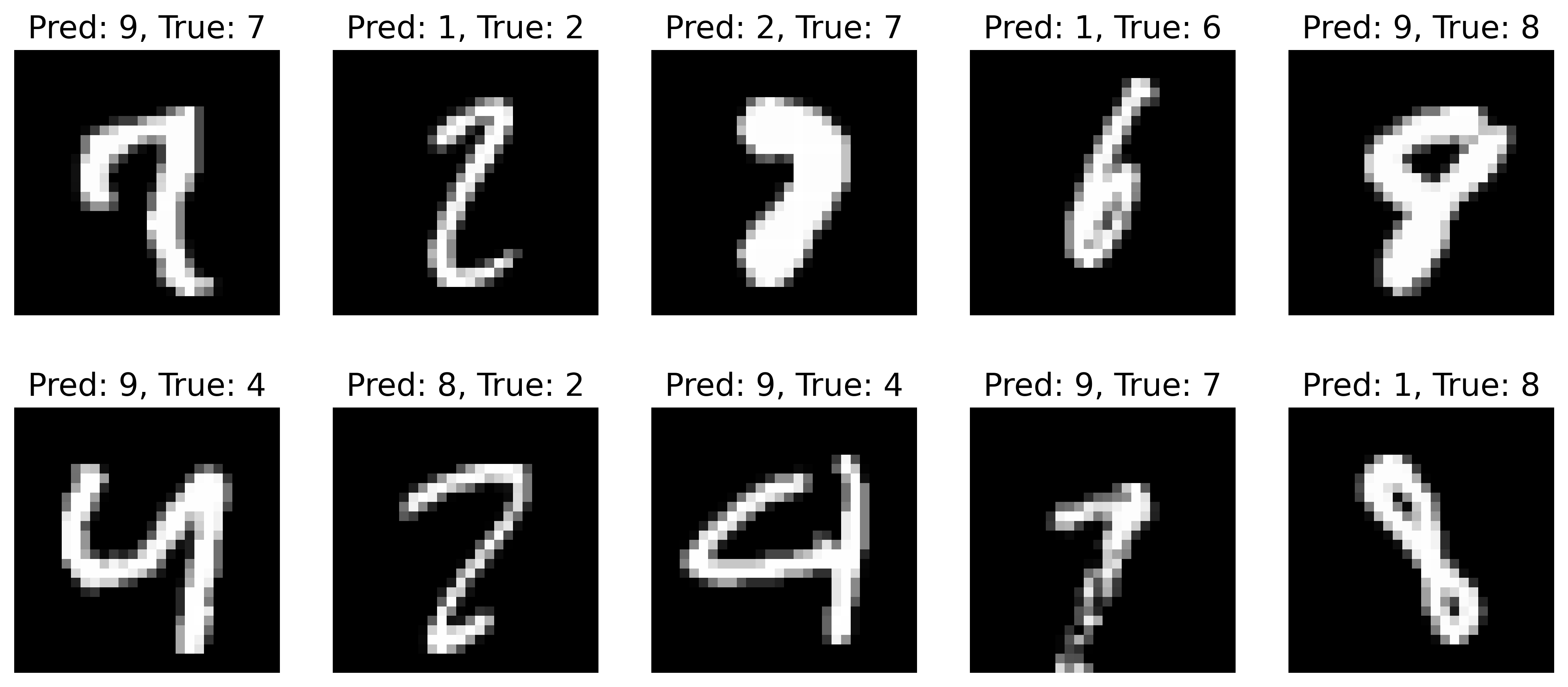
From the image above, we can begin to understand why the model is misclassifying some numbers. The number in the upper left is supposed to be a $7$, but it was written in such a way that it can potentially be confused with a $9$. The number in the upper right is supposed to be an $8$, but it really looks like a $9$. The number $2$ in the bottom row does look like a $2$, but it’s understandable that the model may confuse it with an $8$ since the upper and lower loops look like what someone would do to write an $8$. With the subset of misclassified images we have plotted, it makes sense that the model may struggle with these cases, especially since we only trained it using a small CNN and three total epochs.
Overall, the model does a great job at correctly classifying the MNIST dataset, minus some small subset where the confusion can be attributed to messy numbers. As we saw, training a basic image recognition model is not difficult! Of course, these models are not perfect or fool-proof and with more complex images, we may need more layers, larger layers, or maybe more advanced machine learning techniques.
Feel free to reach out if you have any questions about what we covered this week. Next time, I will show you how to modularize and make improvements to the code. Stay tuned!