Natural language models: DistilBERT sentiment classifier
November 16, 2025
This week, we will be using an encoder to identifying sentiment in movie reviews. First, I will walk through the fine-tuning process. Then, I will show how we use the encoder to identify sentiment with text that the model has not seen.
The classification problem is binary since the sentiment can either be positive or negative. The model we will be fine-tuning, as mentioned in the last post is DistilBERT. Like already discussed, DistilBERT is an encoder that is extracted from a bigger model known as BERT (Bidirectional Encoder Representations from Transformers). Compared to BERT, DistilBERT is about $56$% of the size and $60$% faster, but only retains $97$% of the performance. As is typical with natural language processing (NLP) models, we will be fine-tuning the model weights of an already trained model with a labeled dataset in order to orient the model towards our specific problem. We will use open-source code from Hugging Face, which is a company who has developed libraries for NLP applications and are most known for their transformers library [1].
The first step is defining our parameters. Like previously seen, our parameters will be saved in a .yaml file and we will use SimpleNamespace as an easy way to store and access these parameters. Here are the parameters we will be using:
{
  "model_name": "distilbert-base-uncased",
  "seed": 42,
  "dpi": 400,
  "fig_path": "../outputs/",
  "res_path": "../results/"
}
As can be see, the model name is distilbert-base-uncased. The next step is to load the model and tokenizer. In the Notebook, this is done as follows:
data = "imdb"
dataset = load_dataset(data)

inst = ModelAndTokenizer(cfg.model_name)
model = inst.load_classification_model()
imdb_tokenized = inst.tokenize_dataset(dataset)
Before tokenizing, we much first specify which dataset we are going to be working with. Here, we will be using with the IMDb reviews, which we load using the Hugging Face function load_dataset. We create an instance of our custom class ModelAndTokenizer. This custom class contains methods to used for loading the model, tokenizing the dataset, etc. This class is defined as follows (I will omit the docstrings and unused methods for brevity. See the file model.py for more information):
class ModelAndTokenizer():
    def __init__(
        self,
        model_name: str
    ):
        self.model_name = model_name
        self.device = get_device()
        self.tokenizer: PreTrainedTokenizerBase = AutoTokenizer.from_pretrained(model_name)

    def tokenize_text(
        self,
        prompt: str,
        padding: Union[bool, str] = True,
        truncation: Union[bool, str] = True
    ) -> dict[str, tc.Tensor]:
        inputs = self.tokenizer(
            prompt,
            padding=padding,
            truncation=truncation,
            return_tensors="pt"
        )
        return to_device(inputs, self.device)

    def tokenize_dataset(
        self,
        dataset: Union[Dataset, DatasetDict],
        padding: Union[bool, str] = True,
        truncation: Union[bool, str] = True
    ) -> Union[Dataset, DatasetDict]:
        data_tokenized = dataset.map(
            lambda x: self.tokenizer(
                x["text"],
                padding=padding,
                truncation=truncation
            ),
            batched=True,
            remove_columns=["text"]
        )
        return data_tokenized

    def load_classification_model(
        self,
        attentions: bool = False
    ) -> PreTrainedModel:
        model = AutoModelForSequenceClassification.from_pretrained(
            self.model_name,
            output_attentions=attentions
        ).to(self.device)
        return model
Starting from the top, we see that the input to the class is the model name, in this case distilbert-base-uncased. The load_classification_model method is how we load the model. For encoders, we will use the Hugging Face class AutoModelForSequenceClassification since we will be classifying text. We use the method from_pretrained() to load a pre-trained model, in this case DistilBERT. This method ensures that we also load the model weights. We also include the option of outputting the attentions. These are weights that inform us which are the tokens in a sequence that are more of an influence to specific tokens in that same sequence when processing the data. One can use this information to understand model behavior, token importance, or any model patterns. We also move the model to whatever device we want to use, such as CPU, GPU, etc.
The next step is to tokenize the dataset, which we do using the method tokenize_dataset. This method maps a function to each element of the dataset using a lambda function. The lambda function is what applies the tokenizer to the datset. In this case, it takes x["text"], which is raw text strings, and converts them to tokens. Each sequence is padded to be the same length and the texts that are too long are truncated. The dataset is then batched and the initial x["text"] column is removed (this last step is optional). The output of this method will be a tokenized, batched dataset with labels, input_ids, and attention_mask columns. In our case, the initial dataset was composed of train, test, and unsupervised data with the following structure:
DatasetDict({
    train: Dataset({
        features: ['text', 'label'],
        num_rows: 25000
    })
    test: Dataset({
        features: ['text', 'label'],
        num_rows: 25000
    })
    unsupervised: Dataset({
        features: ['text', 'label'],
        num_rows: 50000
    })
})
Now our tokenized dataset has the following structure:
DatasetDict({
    train: Dataset({
        features: ['label', 'input_ids', 'attention_mask'],
        num_rows: 25000
    })
    test: Dataset({
        features: ['label', 'input_ids', 'attention_mask'],
        num_rows: 25000
    })
    unsupervised: Dataset({
        features: ['label', 'input_ids', 'attention_mask'],
        num_rows: 50000
    })
})
At this point, our dataset is ready to be passed into the encoder.
The next step is to create a training configuration. We do this using the configuration class TrainingArguments where we specify how the model should be trained. In our case we use:
training_args = TrainingArguments(
    output_dir=cfg.res_path,
    overwrite_output_dir=True,
    eval_strategy="epoch",
    save_strategy="epoch",
    logging_strategy="epoch",
    learning_rate=2e-5,
    per_device_train_batch_size=8,
    num_train_epochs=3,
    load_best_model_at_end=True,
)
The first line shows that the output directory where we output the trained model to is res_path, which is defined in our parameters yaml file. The next line specifies that the existing file in the directory will be overwritten by this model. The evaluation will be done every epoch, the checkpoints will be saved every epoch, and metrics logging will be done for every epoch, as well. The learning rate is initialized at $2 \times 10^{-5}$ and the batch size is chosen to be $8$. Overall, the training will be done over three epochs, and once training is done the best model will be loaded. WHile there are many more arguments that can be customized, I only show the basics. I refer you to the Hugging Face documentation for an exhaustive list of the available parameters.
Once our training configuration is complete, we need to set up the training wrapper using Trainer. The Trainer class is a high-level training API provided by Hugging Face that automates the training process. Before, we had to write the training loop, which involved telling PyTorch to calculate the loss function, zero the gradients, propagate the loss, and step the optimizer. Trainer takes care of all the heavy lifting for us under the hood. We initialize the Trainer class as follows:
trainer = Trainer(
    model=model,
    args=training_args,
    train_dataset=imdb_tokenized["train"].shuffle(seed=42).select(range(2000)),
    eval_dataset=imdb_tokenized["test"].shuffle(seed=42).select(range(1000)),
    processing_class=inst.tokenizer,
    compute_metrics=compute_metrics
)
As can be seen, we pass in the model, the training arguments, the different datasets, the tokenizer, and what metrics we want to use (in our case F1 score and accuracy). These datasets are huge so we shuffe, seed, and select a subset of the train ($2000$ samples) and test ($1000$ samples) set as a demonstration. In actual fine-tuning, it’s essential to use all the available data. Now, all we have to do is run trainer.train() and the model begins to train.
For our example, we get the following metrics:
Epoch 	Training Loss   Validation Loss    Accuracy        F1
  1 	   0.430200 	    0.303589 	   0.879000 	0.878852
  2 	   0.196300 	    0.402086 	   0.884000 	0.883926
  3 	   0.115300 	    0.430588 	   0.893000 	0.893013
Overall the metrics look good. The training loss is decreasing per epoch, which is what we are looking for. It also seems exponential, which is a good sign of healthy training. An increasing accuracy over epochs indicates that the model is classifying more examples correctly. The F1 score is also increasing and mirrors the accuracy. This implies that the dataset is balanced and there is no class bias occuring. While the validation loss does increase with each epoch meaning that the model is becoming overconfident and making more incorrect predictions as it trains, the increasing accuracy indicates that the model is still generalizing well. Steps can be taken to mitigate this issue such as early stopping, dropout, and reducing the learning rate.
Once trained, we check to see how well the model classifies the test data by viewing the metrics and plotting a confusion matrix:
{
  "test_loss": 0.32669803500175476,
  "test_accuracy": 0.8633333333333333,
  "test_f1 score": 0.8630762209036968
}
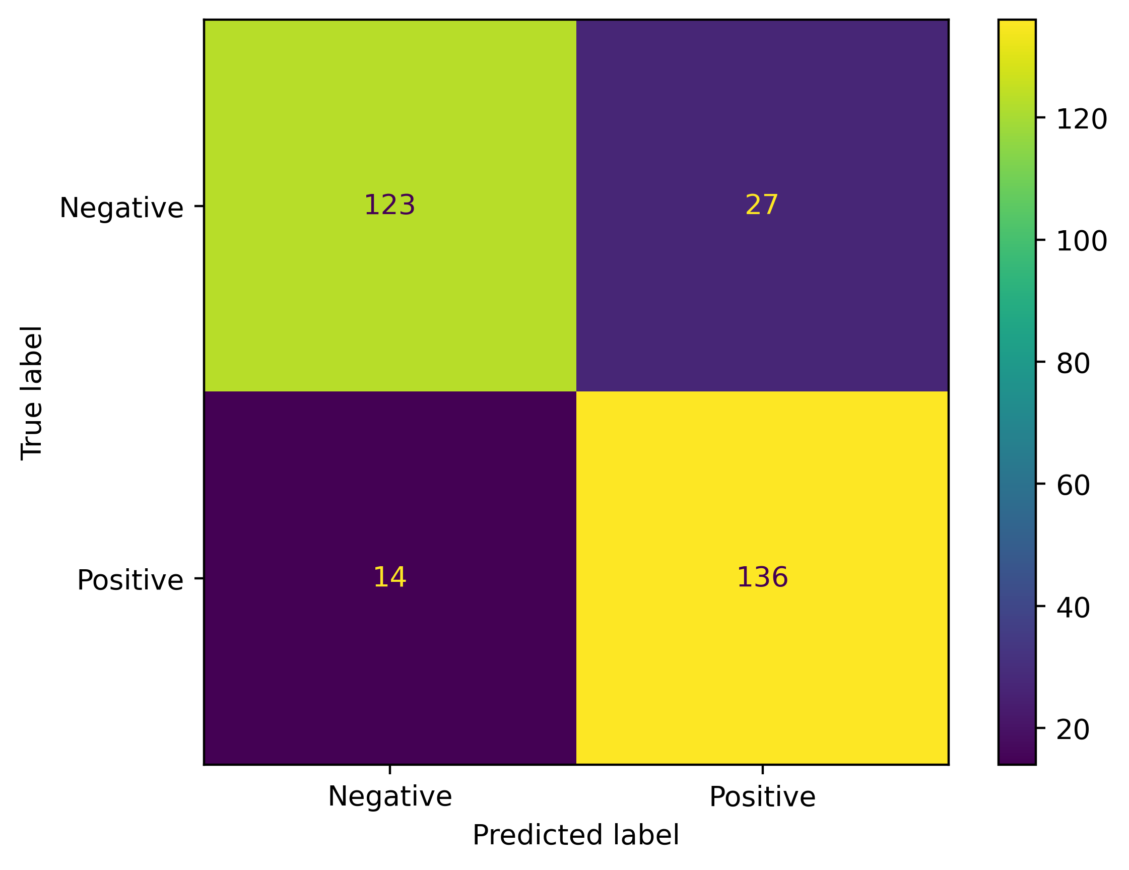
The test metrics are slightly lower, but in the same range as the train metrics, which is a good sign. Plotting a confusion matrix is nice to understand how the predictions are distributed. In this case, the confusion matrix shows that the model is mostly correct in its predictions as the metrics already showed. Our model is now ready to go!
Remember that we are solving a binary classifier problem where sentiment can either be positive or negative so let’s test it on random reviews I generated:
reviews = [
    "That movie was absolutely fantastic!",
    "I will never watch this again!",
    "Highly recommend to never watch again.",
    "Fantastic movie",
    "I kept wondering when it would be over.",
    "You couldn't pay me to watch it again."
]
Judging from the reviews, we can conclude that the first and fourth reviews are positive sentiment, while the rest are negative. Let’s see what the model thinks. First, we tokenize the reviews. Then, we put the model in eval mode, get the outputs, and convert to probabilities:
inputs = inst.tokenize_text(reviews)

model.eval()
with tc.no_grad():
    outputs = model(**inputs)

probs = tc.softmax(outputs.logits.to("cpu"), dim=-1)
predicted_classes = tc.argmax(probs, dim=-1)
labels = ["negative", "positive"]
The results are the following:
Text: 'That movie was absolutely fantastic!'
Probabilities: tensor([0.0520, 0.9480])
Predicted sentiment: positive (0.95 confidence)

Text: 'I will never watch this again!'
Probabilities: tensor([0.7030, 0.2970])
Predicted sentiment: negative (0.70 confidence)

Text: 'Highly recommend to never watch again.'
Probabilities: tensor([0.5231, 0.4769])
Predicted sentiment: negative (0.52 confidence)

Text: 'Fantastic movie.'
Probabilities: tensor([0.1731, 0.8269])
Predicted sentiment: positive (0.83 confidence)

Text: 'I kept wondering when it would be over.'
Probabilities: tensor([0.6879, 0.3121])
Predicted sentiment: negative (0.69 confidence)

Text: 'You couldn't pay me to watch it again.'
Probabilities: tensor([0.8785, 0.1215])
Predicted sentiment: negative (0.88 confidence)
Overall, the model performed well on the reviews. The model managed to correctly predict the sentiment for all the reviews. The first review was very clear in what it was trying to say, hence the high confidence in the positive sentiment classification. The same could be said about the last view when it comes to high confidence in negative sentiment classification.
The third review was borderline, but that’s because of the phrasing. It’s kind of tricky so the model may have a hard time classifying it. In fact, if we run the fine-tuning on different seeds, the third review constantly flips between negative and positive with the probabilities being borderline as they are now. It’s possible that edge cases like this are present in the dataset, which could explain some of the misclassified reviews in the off-diagonal portions of the confusion matrix plot. I would surmise that if we fine-tuned the model with the full training dataset, instead of just a subset, we may have been able to lower the values in the off-diagonal. Regardless, the values are small compared to the diagonal, so the subset chosen is good enough for our application.
We have managed to fine-tune a DistilBERT model to predict sentiment in movie reviews. To summarize, we have walked through the process of fine-tuning an encoder to perform a specific task, which was classify movie reviews. The process involved importing the pre-trained language model, tokenizing the dataset, setting up the training arguments and the Trainer class, fine-tuning the model, then seeing how well the model performs with unseen data. We then made up reviews, with one curveball in the mix, and the model managed to correctly classify them. Overall, we have now learned about encoders, how to fine-tune one for a specific task, and produced a model that performed well on a binary classification problem.
The code and plot presented in this post can be found on my Github under the nlp-model repo [2]. Feel free to reach out if you have any questions about what we covered this week. Next week we will move on to decoders. Stay tuned!
- [1] Thomas Wolf, Lysandre Debut, Victor Sanh, et al., HuggingFace’s Transformers: State-of-the-art Natural Language Processing, 2020. Available at: https://arxiv.org/abs/1910.03771.
- [2] Alberto J. Garcia, NLP Model, 2025. Available at: https://github.com/AJG91/nlp-model.