Charged Particle Dynamics: Numerical Results
November 15, 2026
This week I will introduce two numerical integrators, discuss some of their properties, develop a simulation of a particle in a specific electromagnetic field configuration, and analyze the results. We will be using the integrators to solve the equations introduced in the previous post.
Computational Methods
In order to solve the Lorentz force equation numerically, we must implement an integrator. First, let’s rewrite the Lorentz force,
\[\deriv{v_i}{t} = \frac{q}{m} (E_i + \levi{i}{j}{k} v_j B_k). \label{eq:em_force_vel} \tag{1}\]Now, I will go over a few numerical integrator options:
Forward Euler Method
This is a first-order method and is considered to be the most basic method for numerical integration of differential equations. Since it is first-order, the truncation error is second-order. We can derive the method by applying a Taylor expansion of $y(t)$ about $t_n$
Defining $y_{n+1} = y(t_n + \delta t)$ and substituting in the general form of a first-order differential equation, $y^\prime(t_n) = f(t_n, y_n)$ yields
\[y_{n+1} \approx y(t_n) + \delta t f(t_n, y_n).\]This approximation has a first-order global error since it’s linear, which is why it’s known as a first-order method.
Let’s understand how the energy behaves with this integrator. Referring back at $\text{Eq.}~\eqref{eq:em_force_vel}$ and assuming $\E = 0$ and $\B$ is constant, we can write
\[\vvec_{n+1} = \vvec_n + \frac{q \Delta t}{m} (\vvec_n \times \B). \label{eq:vel_forward_step_general} \tag{2}\]The change in kinetic energy between timesteps can also be written as
\[K_{n+1} - K_n = \frac{1}{2}m \Big(\lVert \vvec_{n+1} \rVert^2 - \lVert \vvec_{n} \rVert^2\Big). \label{eq:kinetic_energy_diff} \tag{3}\]Then, the $\vvec_{n+1}$ term becomes
\[\lVert \vvec_{n+1} \rVert^2 = \lVert \vvec_{n} \rVert^2 + \Big(\frac{q \Delta t}{m}\Big)^2 \lVert \vvec_{n} \times \B \rVert^2, \label{eq:vel_forward_step} \tag{4}\]where the cross term cancels out since the dot product is zero. Now, $\text{Eq.}~\eqref{eq:kinetic_energy_diff}$ becomes
\[K_{n+1} - K_n = \frac{1}{2} \frac{q^2 \Delta t^2}{m} \lVert \vvec_{n} \times \B \rVert^2 \ge 0. \label{eq:diff_kinetic_energy} \tag{5}\]From $\text{Eq.}~\eqref{eq:diff_kinetic_energy}$, we conclude that the kinetic energy will always increase with each consecutive time step. This is not a physical property, but a numerical property brought on by the intergrator we chose. We can also determine the overall shape of the kinetic energy over time. To do this, we split the velocity into the parallel and perpendicular components and plug them into the kinetic energy
\[K_n = \frac{1}{2}m \Big(\lVert \vvec_{\parallel, n} \rVert^2 + \lVert \vvec_{\perp, n} \rVert^2\Big), \label{eq:kinetic_energy_para_perp_vel} \tag{6}\]where the cross terms cancel since $\vvec_{\parallel, n} \cdot \vvec_{\perp, n} = 0$. We can now focus on the $\vvec_{\perp, n}$ terms since the parallel terms conserve energy throughout the trajectory. Thus,
\[K_{\perp, n} = \frac{1}{2}m \lVert \vvec_{\perp, n} \rVert^2, \label{eq:kinetic_energy_perp_vel} \tag{7}\]We can also write $\text{Eq.}~\eqref{eq:vel_forward_step}$ in terms of the components,
\[\lVert \vvec_{\parallel, n+1} + \vvec_{\perp, n+1} \rVert^2 = \big(\vvec_{\parallel, n} + \vvec_{\perp, n}\big) + \Big(\frac{q \Delta t}{m}\Big)^2 \lVert \big(\vvec_{\parallel, n} + \vvec_{\perp, n}\big) \times \B \rVert^2.\]Cancelling out the dot product between velocities and cross product between $\vvec_{\parallel, n}$ and $\B$, and substituting for the cyclotron frequency, we obtain
\[\begin{aligned} \lVert \vvec_{\parallel, n+1} \rVert^2 ={}& \lVert \vvec_{\parallel, n} \rVert^2, \\ \lVert \vvec_{\perp, n+1} \rVert^2 ={}& \Big(1 + \Delta t^2 \omega^2_c \Big) \lVert \vvec_{\perp, n} \rVert^2. \end{aligned}\]As with $\text{Eq.}~\eqref{eq:diff_kinetic_energy}$, these equations also show that the kinetic energy has to increase. Focusing on the perpendicular term, by taking consequtive timesteps, we can show that the following relationship holds:
\[\lVert \vvec_{\perp, n+1} \rVert^2 = \Big(1 + \Delta t^2 \omega^2_c \Big)^{t / \Delta t+1} \lVert \vvec_{\perp, 0} \rVert^2.\]With this equation and the kinetic energy equation, we can write
\[K_{\perp, n} = \Big(1 + \Delta t^2 \omega^2_c \Big)^{t / \Delta t} K_{\perp, 0},\]where we have shifted $n$ by one without loss of generality. Taking the natural log of both sides yields
\[\ln\Bigg( \frac{K_{\perp, n}}{K_{\perp, 0}} \Bigg) = \frac{t}{\Delta t} \ln \Big(1 + \Delta t^2 \omega^2_c \Big).\]If $\Delta t^2 \omega^2_c \ll 1$, we can expand the natural log,
\[\ln\Bigg( \frac{K_{\perp, n}}{K_{\perp, 0}} \Bigg) = \frac{t}{\Delta t} \Big(\Delta t^2 \omega^2_c \Big),\]and thus
\[K_{\perp, n} \approx K_{\perp, 0}\exp^{t \Delta t \omega^2_c}. \label{eq:euler_ke} \tag{8}\]From $\text{Eq.}~\eqref{eq:euler_ke}$, we can draw the conclusion that as time goes on, the kinetic energy calculated from Euler method solutions will increase exponentially. Likewise, for small timesteps, the kinetic energy will increase linearly. This tells us that while the Euler method may provide decent solutions for small values of $\Delta t$ and short time periods, the kinetic energy will greatly increase as larger values of $\Delta t$ are chosen and/or for large time periods, which will result in an increasing inaccuracy in the Forward Euler method solutions.
Runge-Kutta Method
The Runge-Kutta Method is one of the most well-known algorithms used to solve ordinary differential equation. The most common version of the Runge-Kutta method is the fourth-order Runge-Kutta (a.k.a. RK4). For comparisons, the Forward Euler Method is a first-order Runge-Kutta method. I’ll only list the method here.
The implementation of the RK4 is as follows:
For $y^\prime = f(y)$,
\[y_{n+1} = y_n + \frac{\Delta t}{6} (k_1 + 2 k_2 + 2 k_3 + k_4), \label{eq:rk4_eq} \tag{9}\]where
\[\begin{align} k_1 ={}& f(y_n), \\ k_2 ={}& f\Big(y_n + \frac{\Delta t}{2}k_1\Big), \\ k_3 ={}& f\Big(y_n + \frac{\Delta t}{2}k_2\Big), \\ k_4 ={}& f(y_n + \Delta t k_3). \end{align}\]Just like with the Forward Euler method, we can show how the energy behaves when utilizing this integrator. We write $\text{Eq.}~\eqref{eq:em_force_vel}$ as
\[A\vvec = \frac{q}{m} \vvec \times \B, \label{eq:lorentz_force_operator} \tag{10}\]where $A$ is a linear operator, thus
\[\deriv{\vvec}{t} = A\vvec.\]Here, $A^T = -A$ due to the property of the cross product. Let’s write out the RK4. Since we assume $\E = 0$ and $\B$ is constant, the different $k$ values take the following form:
\[\begin{aligned} k_1 ={}& A\vvec_n, \\ k_2 ={}& A\vvec_n + A^2 \frac{\Delta t}{2} \vvec_n, \\ k_3 ={}& A\vvec_n + A^2 \frac{\Delta t}{2} \vvec_n + A^3 \frac{\Delta t^2}{4} \vvec_n, \\ k_4 ={}& A\vvec_n + A^2 \frac{\Delta t}{2} \vvec_n + A^3 \frac{\Delta t^2}{4} \vvec_n + A^4 \frac{\Delta t^3}{4} \vvec_n. \end{aligned}\]Plugging these into $\text{Eq.}~\eqref{eq:rk4_eq}$ and simplifying, we obtain
\[\vvec_{n+1} = \Big(\mathbf{I} + \Delta t A + \frac{\Delta t^2}{2!}A^2 + \frac{\Delta t^3}{3!}A^3 + \frac{\Delta t^4}{4!}A^4 \Big) \vvec_n. \label{eq:rk4_vel_expansion} \tag{11}\]For simplicity, we can write $\text{Eq.}~\eqref{eq:rk4_vel_expansion}$ as
\[\vvec_{n+1} = \Lambda \vvec_n, \label{eq:rk4_vel_expansion_operator} \tag{12}\]where $\Lambda$ is a linear operator. We now take $\text{Eq.}~\eqref{eq:kinetic_energy_diff}$ and substitute $\text{Eq.}~\eqref{eq:rk4_vel_expansion_operator}$, which yields
\[K_{n+1} - K_n = \frac{1}{2}m \vvec^T_n \big(\Lambda^T\Lambda - \mathbf{I} \big)\vvec_n.\]We can work out the distribution of $\Lambda^T\Lambda$ by using the fact that $A^T = -A$. This works out to be
\[\Lambda^T\Lambda - \mathbf{I} = \frac{\Delta t^6}{72}A^6 + \frac{\Delta t^8}{576}A^8,\]which then gives
\[K_{n+1} - K_n = \frac{1}{2}m \vvec^T_n \Big(\frac{\Delta t^6}{72}A^6 + \frac{\Delta t^8}{576}A^8 \Big)\vvec_n. \label{eq:kinetic_energy_diff_rk4} \tag{13}\]Now, we must work out what the different powers of $A$ are. Going back to $\text{Eq.}~\eqref{eq:lorentz_force_operator}$, we multiply both sides by $A$,
\[\begin{split} A(A\vvec) ={}& \frac{q}{m} (A\vvec) \times \B = \frac{q}{m} \Big[\frac{q}{m}\vvec \times \B \Big] \times \B, \\ ={}& \frac{q^2}{m^2} \Big[\B(\vvec \cdot \B) - \vvec (\B \cdot \B) \Big]. \end{split}\]We multiply both sides by $A$ once more,
\[\begin{split} A(A^2\vvec) ={}& \frac{q^3}{m^3} \Big[\B(\vvec \cdot \B) - \vvec (\B \cdot \B) \Big] \times \B, \\ ={}& \frac{q^3}{m^3} \Big[(\vvec \cdot \B) (\B \times \B) - (\B \cdot \B) (\vvec \times \B) \Big], \\ ={}& -\frac{q^3}{m^3} B^2 (\vvec \times \B), \\ ={}& -\frac{q^2 B^2}{m^2} \Big[\frac{q}{m} (\vvec \times \B)\Big]. \end{split}\]Substituting in for the cyclotron frequency and recognizing that we’re obtained $\text{Eq.}~\eqref{eq:lorentz_force_operator}$ once again, we can write
\[A^3\vvec = -\omega^2_c A\vvec.\]This relationship implies that
\[A^8\vvec = -\omega^2_c A^6\vvec\]since we can multiply both sides by $A^5$. $\text{Eq.}~\eqref{eq:kinetic_energy_diff_rk4}$ then becomes
\[K_{n+1} - K_n = \frac{m \Delta t^6}{144} \Big(1 - \frac{\omega^2_c\Delta t^2}{8}\Big)\vvec^T_n A^6 \vvec_n. \label{eq:kinetic_energy_diff_rk4_with_A} \tag{14}\]The combination of $\vvec$ and $A$ can be written as
\[\vvec^T_n A^6 \vvec_n = -(A^3 \vvec_n)^T(A^3 \vvec_n) = -\lVert A^3 \vvec_n \rVert^2 = \omega^4_c \Big\lVert \frac{q}{m} (\vvec_n \times \B) \Big\rVert^2,\]thus,
\[K_{n+1} - K_n = -\frac{m \omega^4_c \Delta t^6}{144} \Big(1 - \frac{\omega^2_c\Delta t^2}{8}\Big) \Big\lVert \frac{q}{m} (\vvec_n \times \B) \Big\rVert^2.\]We can now separate out the velocity in terms of parallel and perpendicular components. Since the parallel component crossed with the magnetic field is zero, we are left with
\[K_{n+1} - K_n = -\frac{m \omega^6_c \Delta t^6}{144} \Big(1 - \frac{\omega^2_c\Delta t^2}{8}\Big) \lVert \vvec_{\perp, n} \rVert^2. \label{eq:rkfour_ke} \tag{15}\]From $\text{Eq.}~\eqref{eq:rkfour_ke}$, we can consider multiple cases:
- Case 1: $\frac{\omega^2_c\Delta t^2}{8} = 1$,
- Case 2: $\frac{\omega^2_c\Delta t^2}{8} > 1$,
- Case 3: $\frac{\omega^2_c\Delta t^2}{8} < 1$.
For case 1, $\text{Eq.}~\eqref{eq:rkfour_ke}$ becomes $K_{n+1} = K_n$ and we obtain conservation of energy. Note that while the kinetic energy is conserved, this does not mean that the trajectory is correct since the direction of the velocity is not accounted for in $\text{Eq.}~\eqref{eq:rkfour_ke}$. Another way for the system to conserve energy would be if $\vvec_{\perp, n} = 0$. This would mean that the particle only has parallel velocity, which corresponds to a constant planar velocity (hence conservation of energy) as discussed in the blog post last week.
For case 2, we would get an increasing kinetic energy as time passes. As with the Forward Euler method, this is not a physical property, but a numerical property brought on by the intergrator we chose. The RK4 solution is unstable due to either a large cyclotron frequency or a large timestep, which introduces a small error in the form of a numerical increase in the perpendicular velocity at every timestep. For both scenarios, the timestep has to be adjusted to correctly account for the motion caused by the magnetic field, thus moving the system towards case 1 or 3. If the timestep is too large, then the gyration will not be properly accounted for, causing the RK4 to provide an inadequate solution.
For case 3, we obtain a decreasing kinetic energy as time moves forward. This implies that the integrator is not reproducing the exactly circular trajectory, but instead introduces a small error in the form of a numerical reduction in the perpendicular velocity at every timestep. As before, this is not a physical property, but a numerical property brought on by the intergrator we chose. Note that for relatively short time periods this is not an issue and the RK4 provides a very good solution. A decreasing perpendicular velocity will only be apparent in the RK4 solutions if we take thousands of iterations.
Results
We will be solving the Lorentz force equation for a charged particle in a specific electromagnetic field configuration. The initial conditions are:
- $\xvec_0 = \langle 0, 0, 0 \rangle$ [m],
- $\vvec_0 = \langle 1, 0, 0 \rangle$ [m/s],
- $\E = \langle 0, 0, 0 \rangle$ [N/C],
- $\B = \langle 0, 0, 1 \rangle$ [T].
We assume normalized units, i.e., $q = 1$ and $m = 1$. The timesteps we will use are $\Delta t = [0.1, 0.05, 0.01, 0.005]$ and the simulation will run over $4$ cycles.
In Fig. 1 we show the exact and numerical solutions to the Lorentz force and the gyro-motion for timestep $dt = 0.01$ using the Forward Euler method integrator. The top row shows the position, the middle row the velocity, and the bottom row the absolute error between the exact solution and the numerical solution from the Euler method. In Fig. 2, we show the same quantities, but for timestep $dt = 0.1$.
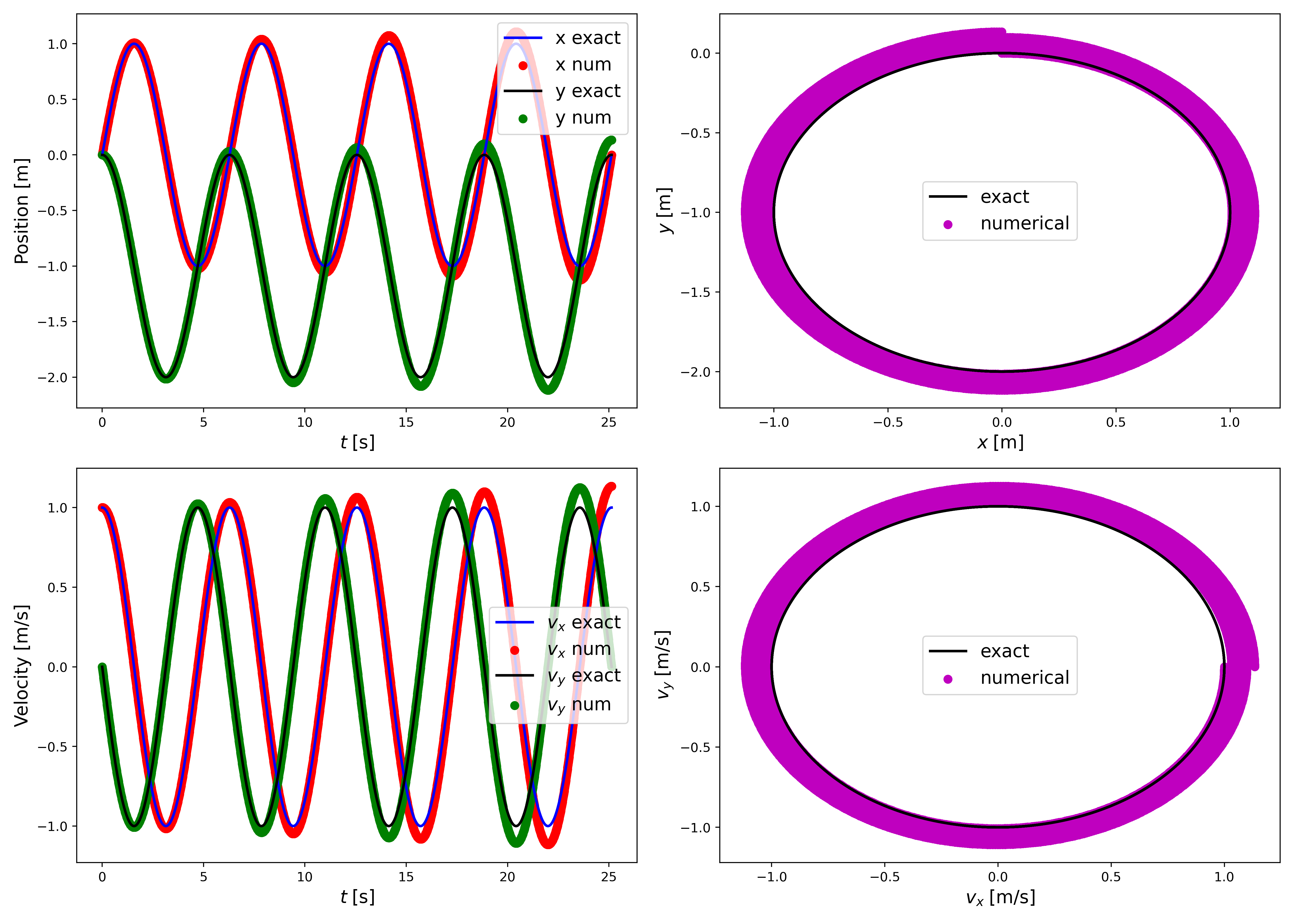
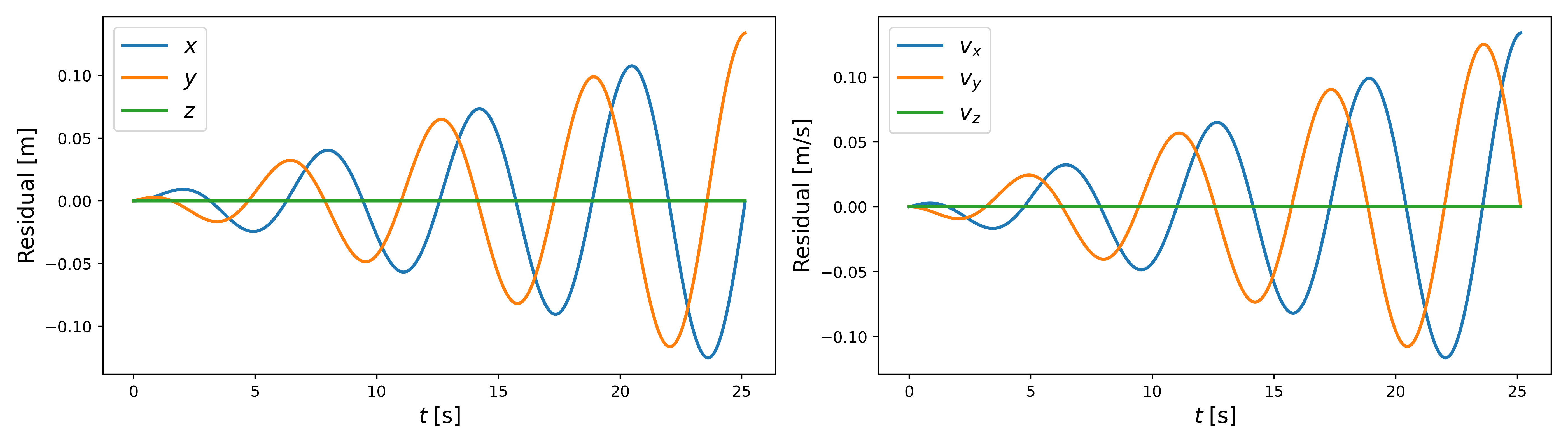 Figure 1: Euler method solutions with errors with timestep $dt = 0.01$.
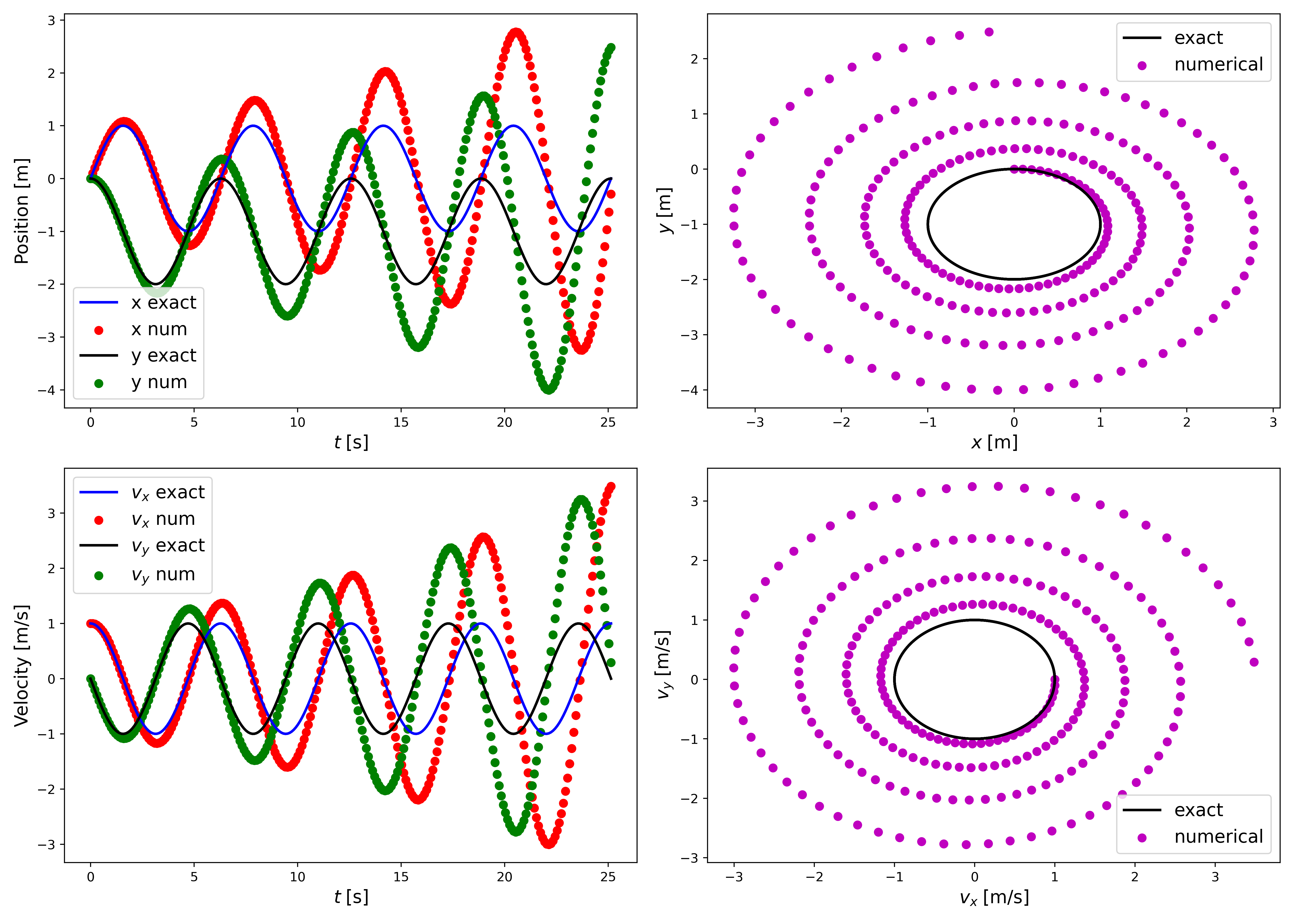
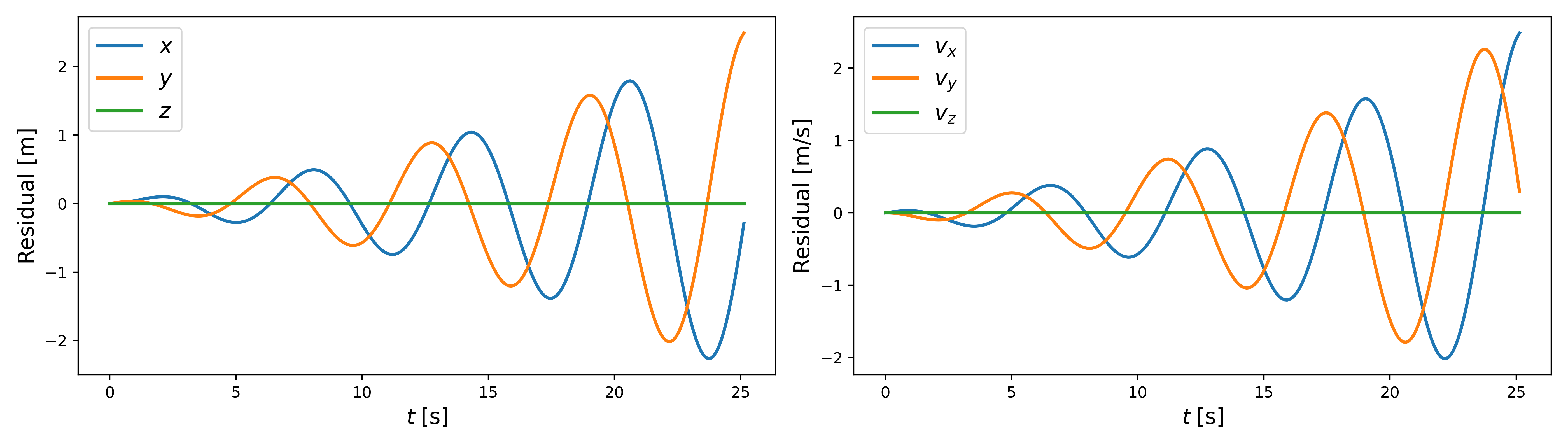 Figure 2: Euler method solutions with errors with timestep $dt = 0.1$.
As discussed in Computational Methods, the Forward Euler method begins to lose accuracy as time goes on. This is evident from the plots on the left that show the position and velocity versus time. Initially, the position starts off well-approximated, but as more cycles are completed, the numerical velocity and position solutions begin to overshoot the exact solution. This is also evident by the plots on the right that show $y$ vs. $x$ and $v_y$ vs. $v_x$. The particle begins to spiral out of the expected circular trajectory. As the timestep increases, the inaccuracies greatly increase and the particle completely leave the exact trajectory. If we look at the bottom row of plots, the signed residual oscillates and the amplitudes of the oscillations slowly start growing as the particle travels more cycles.
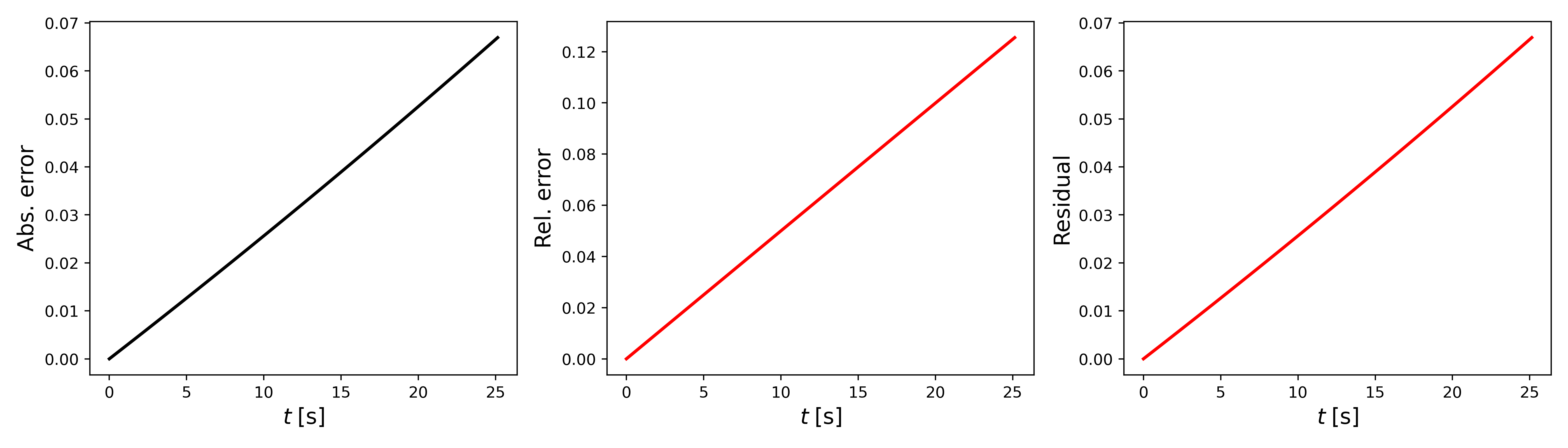
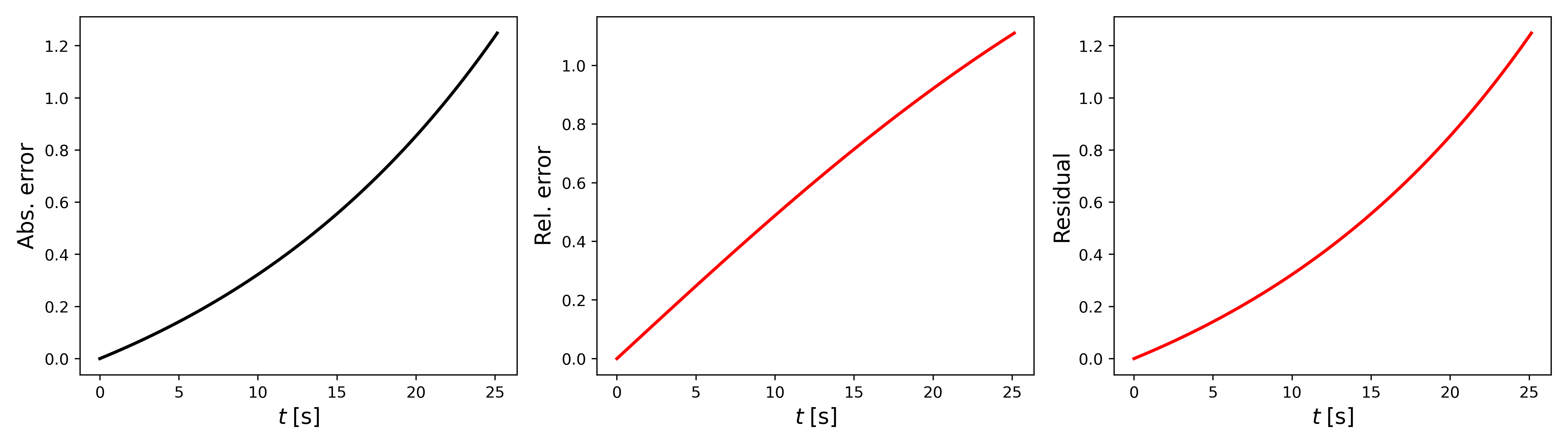 Figure 3: Kinetic energy calculated using the Euler method solutions for two different timesteps: (top) $dt = 0.01$ and (bottom) $dt = 0.1$.
In Fig. 3, we show the absolute, relative, and residual error of the kinetic energy calculated using the Forward Euler method integrator for both timesteps: (top) $dt = 0.01$ and (bottom) $dt = 0.1$. The residual error is signed, as opposed to the absolute and relative errors. As discussed in Computational Methods, the kinetic energy increases as times goes on. For the smaller timestep (top plots), the kinetic energy appears linear. For the larger timestep (bottom plots), the kinetic energy now takes an increasing exponential form. This is exactly what we derived from the Forward Euler method integrator. The absolute and relative errors show the same conclusion.
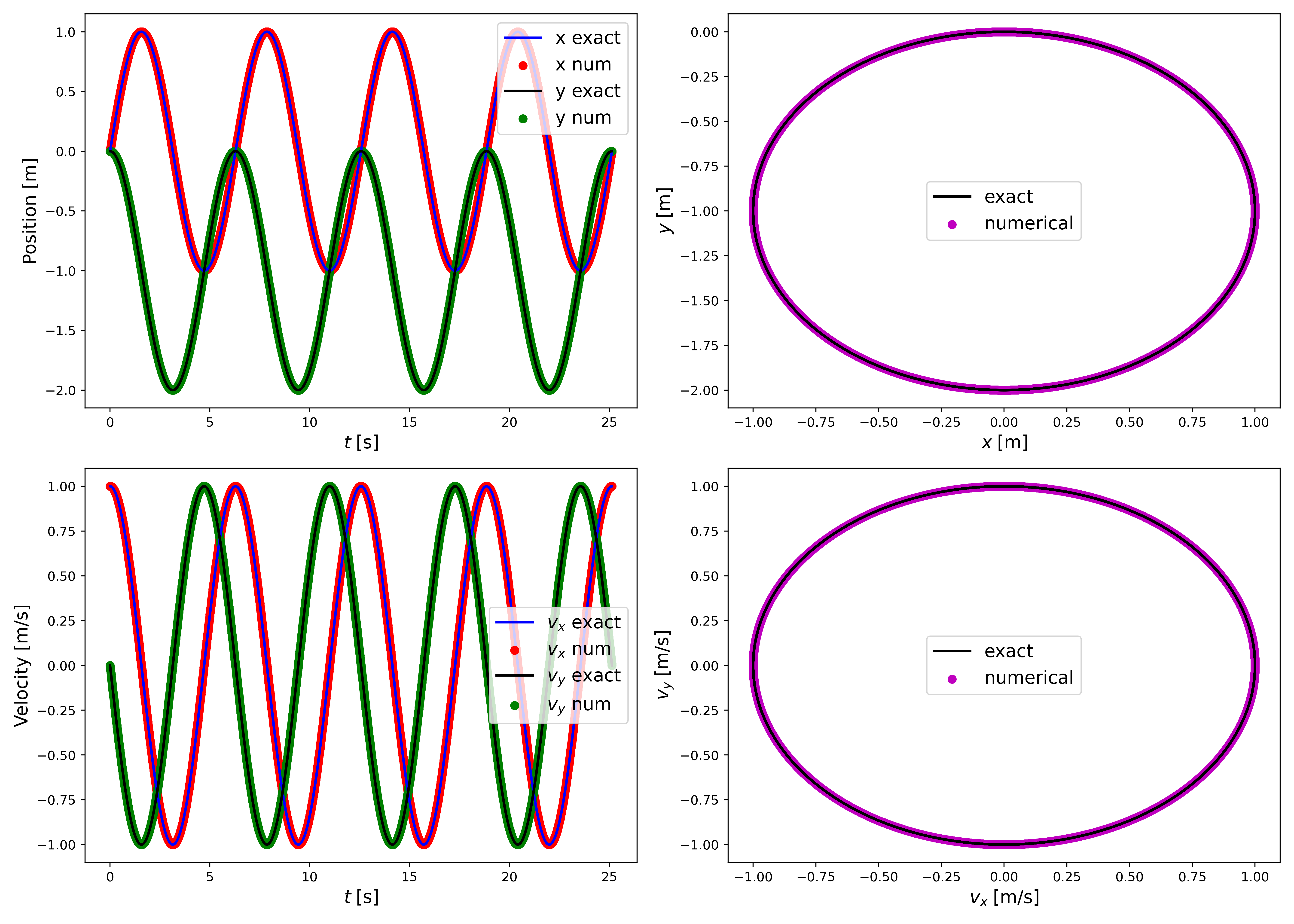
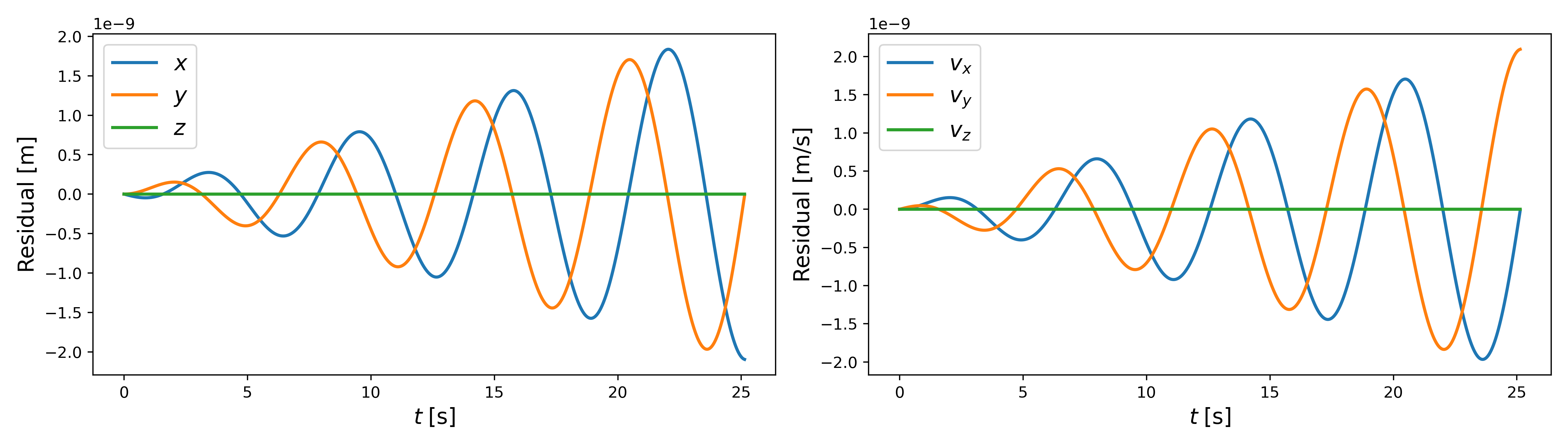 Figure 4: RK4 method solutions with errors with timestep $dt = 0.01$.
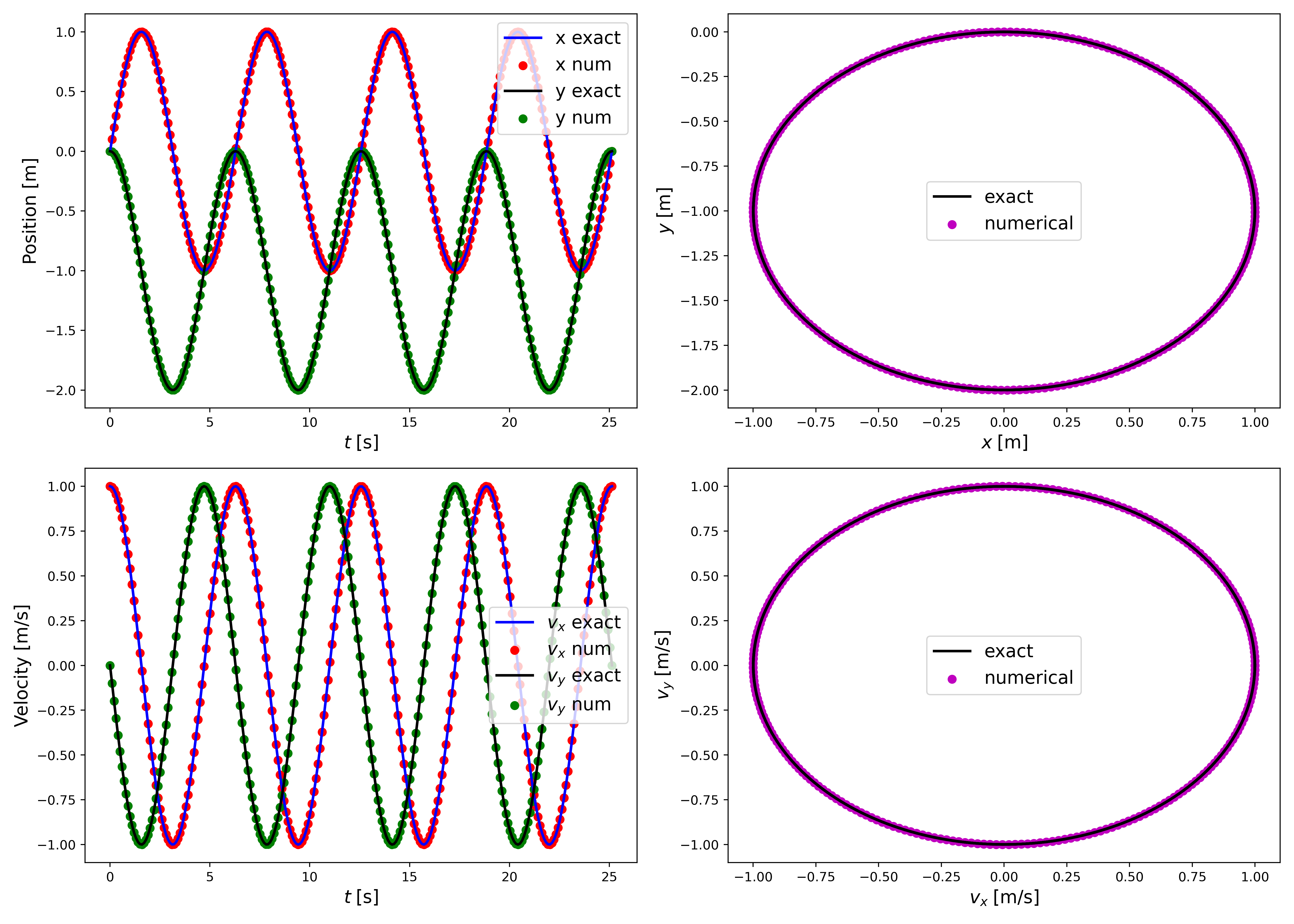
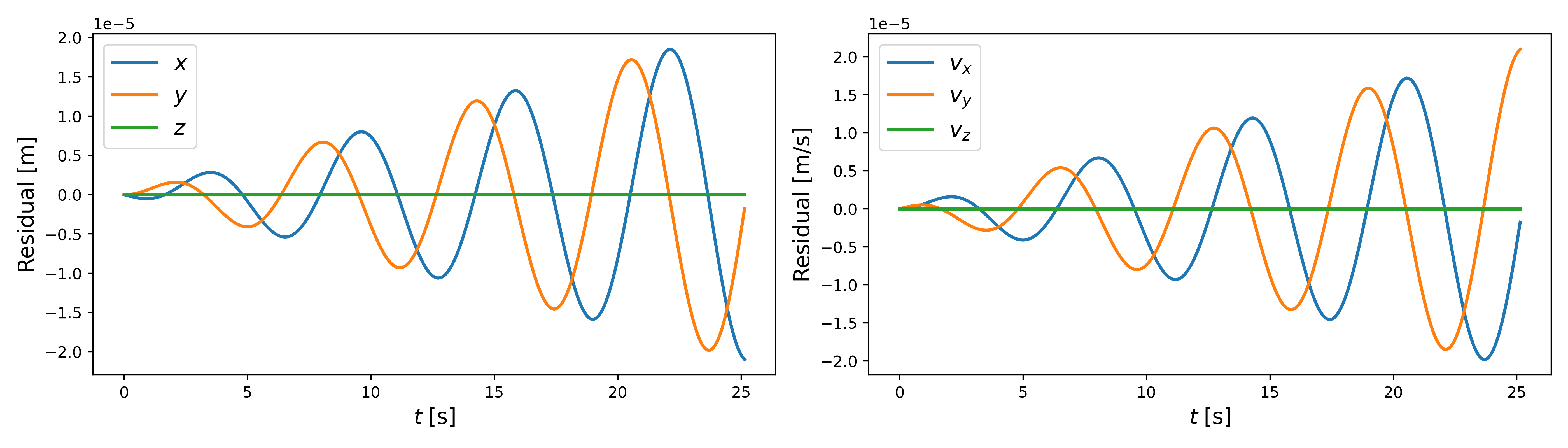 Figure 5: RK4 method solutions with errors with timestep $dt = 0.1$.
In Fig. 4, we show the exact and numerical solutions to the Lorentz force and the gyro-motion for timestep $dt = 0.01$ using the RK4 integrator. The top row shows the position, the middle row the velocity, and the bottom row the absolute error between the exact solution and the numerical solution from the RK4 method. In Fig. 5, we show the same quantities, but for timestep $dt = 0.1$.
As discussed in Computational Methods, the RK4 method provides stable solutions for our system throughout the time period we chose. The absolute errors are on order of $10^{-9}$ for timestep $dt = 0.01$. For the timestep $dt=0.1$, the absolute errors do fall to $10^{-5}$. Although the solutions are still fairly accurate, this decrease in accuracy is exactly what we predicted in Computational Methods as the timestep increases.
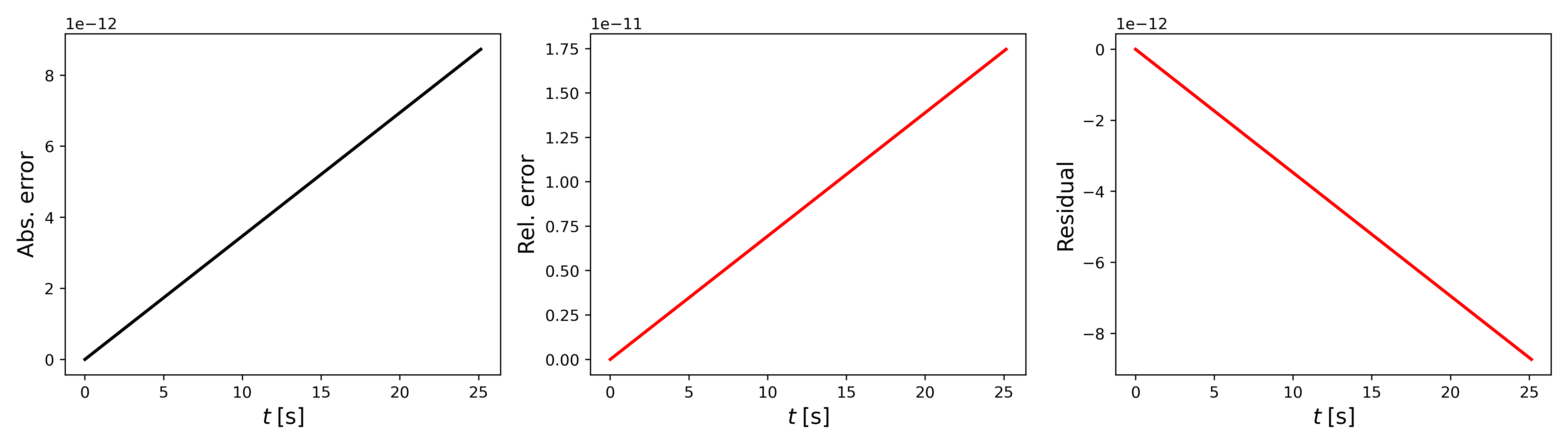
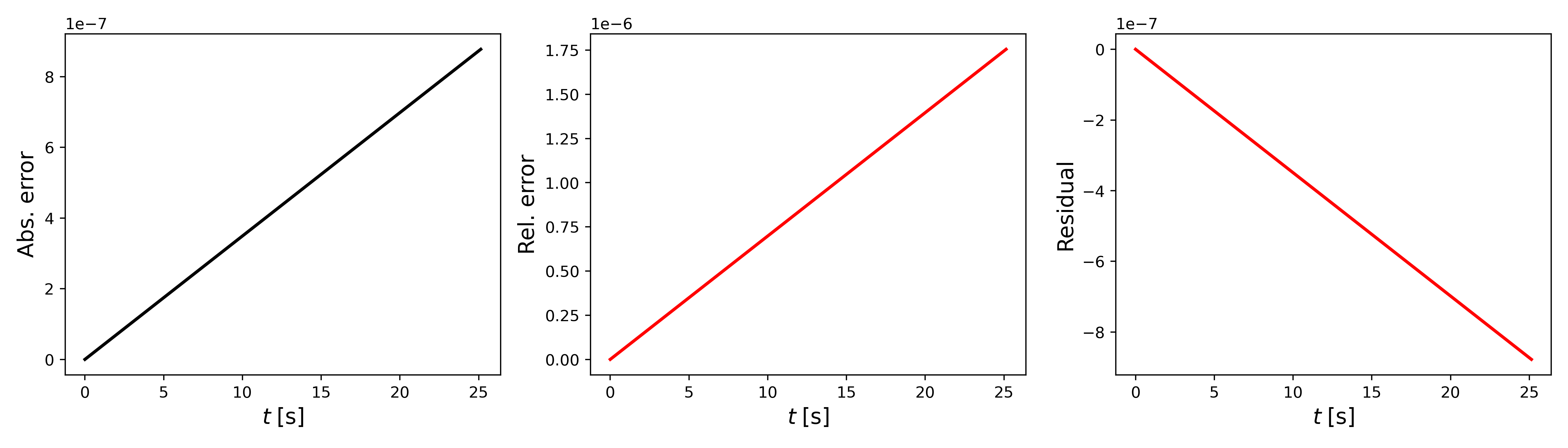 Figure 6: Kinetic energy calculated using the RK4 method solutions for two different timesteps: (top) $dt = 0.01$ and (bottom) $dt = 0.1$.
In Fig. 6, we show the absolute, relative, and residual error of the kinetic energy calculated using the RK4 method integrator for both timesteps: (top) $dt = 0.01$ and (bottom) $dt = 0.1$. As previously mentioned, the residual error is signed, as opposed to the absolute and relative errors. From the plots, we see that the kinetic energy does indeed decrease with consecutive time steps. As we predicted, the accuracy decreases as we increase the timestep. The error for the timestep $dt = 0.01$ is on the order of $10^{-12}$, while the error for the timestep $dt = 0.1$ is on the order of $10^{-7}$. This shows that the RK4 provides much more accurate solutions compared to the Forward Euler method.
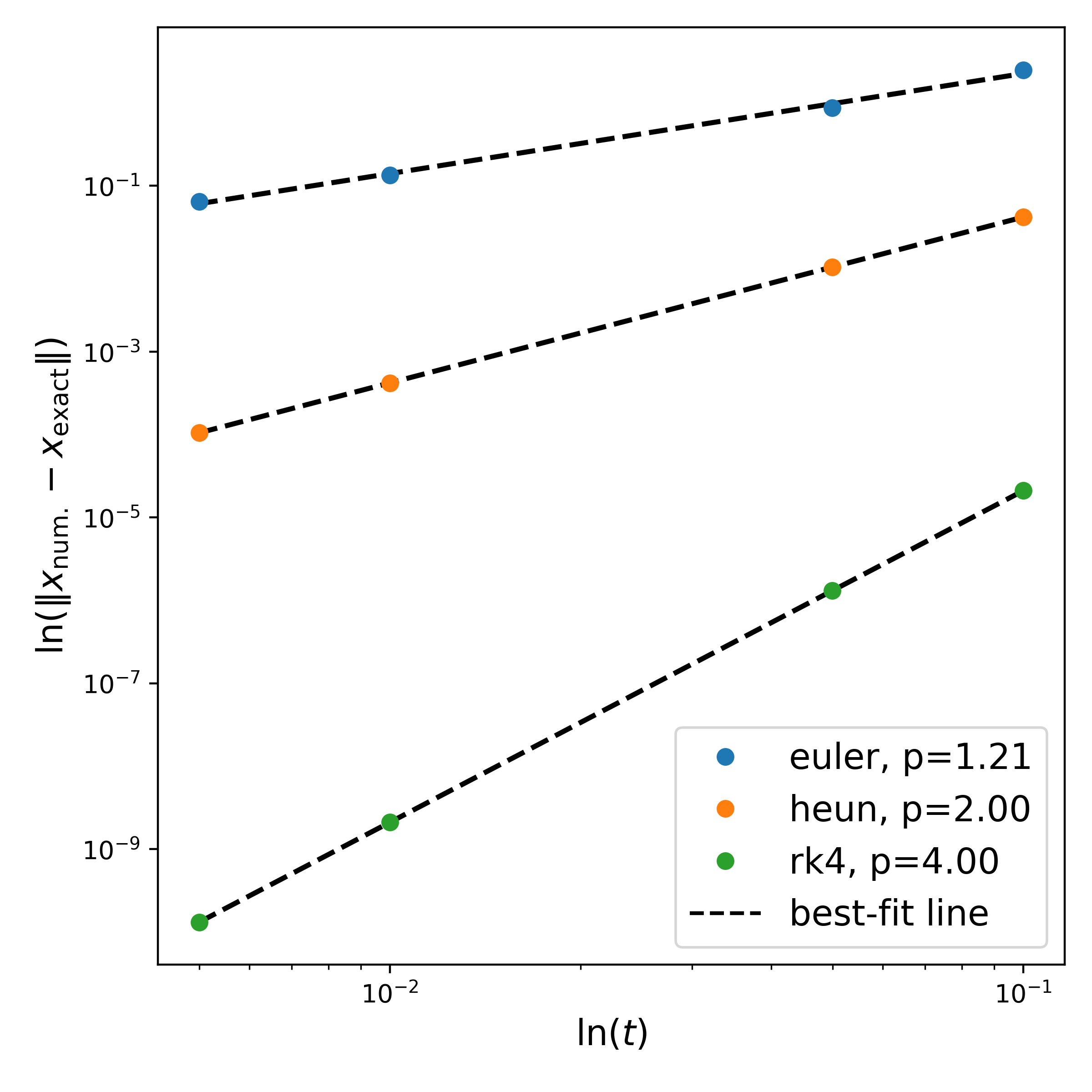 Figure 7: Integrator convergence.
In Fig. 7, we show the convergence of the different integrators. For comparison purposes, we also included an additional integrator known as the Heun method. This is a second-order method that improves upon the Euler method and can be derived from the general RK4 method. The figure plots the natural logarithm of the maximum positional error versus the natural logarithm of the timestep size to determine the specified numerical method’s order of convergence. We have also drawn a best-fit line.
In general, the slope of the best-fit line in log-log space should be $\sim 1$ for a first-order method, $\sim 2$ for a second-order method, and $\sim 4$ for a fourth-order method. From the figure, we see that the best-fit lines for the Heun and RK4 methods do in fact have the appropriate slopes, which we denote as $p$. On the other hand, the slope of the best-fit line for Euler’s method is not quite $1$, but this is due to the inaccuracies introduced due to the timestep size and the number of cycles as we discussed in Computational Methods and as the error plots have shown. Overall, these results confirm that our integrators work as expected.
Summary
We have introduced two different integrators for solving differential equations and explored some of their properties. We developed a simulation of a charged particle in a specific electromagnetic field configuration and solved the Lorentz force over different timesteps and analyzed the results. Finally, we plotted the convergence of the different integrators to verify that they were working correctly.
Overall, we verified that our simulation accurately reproduced the physical behavior predicted by our theoretical derivations. We also confirmed that the integrators exhibited the expected properties. These results provide a solid foundation for applying these numerical methods to more complex physical systems in future simulations.
The code presented in this post can be found on my Github under the charged-particle-dynamics repo [1]. A PDF version of these this and last week’s post can be found in Ch. 1 of my computational plasma physics notes. Feel free to reach out if you have any questions about what we covered this week. Stay tuned for the next topic!
- [1] Alberto J. Garcia, The Dynamics of a Charged Particle in an Electromagnetic Field, 2026. Available at: https://github.com/AJG91/charged-particle-dynamics.